Week 3 - Solving second order ODEs

AIM-

• Solving ODE equation of Simple Pendulum with damping.

OBJECTIVE-

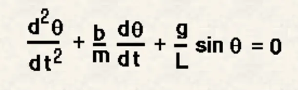
• To write a program that solves the following ODE. This ODE represents the equation of motion of a simple Pendulum with damping.
• 

THEORY-

Newton’s second low of motion-

• The rate of change of linear momentum of a body is directly proportional to the external force applied on the body, and this change takes place always in the direction of the force applied.

Simple Pendulum-

• Simple Pendulum is a mechanical device demonstrating periodic motion.
• This has a small circular bob suspended by a thin inextensible string from any fixed end and has length L.
• Oscillatory motion – Any to and for motion performed by the pendulum in a periodic movement and when the pendulum is at its central position then the position is called equilibrium position.
• Time period – It is generally the total time taken by a pendulum to complete one full oscillation.
• Amplitude – The distance between the equilibrium position and the extreme position of the pendulum.
• Length – Length of the string is generally the distance between the fixed end of a string to the center of mass.

In the above equation,

g = gravity in m/s2,

L = length of the pendulum in m,

m = mass of the ball in kg,

b=damping coefficient.

Write a program in python that will simulate the pendulum motion, just like the one shown in the start of this challenge.

use,

L=1 metre,

m=1 kg,

b=0.02

g=9.81 m/s2.

Simulate the motion between 0-20 sec, for angular displacement=0,angular velocity=3 rad/sec at time t=0.

PROGRAM

import numpy as np
from scipy.integrate import odeint
import matplotlib.pyplot as plt
import math
from PIL import Image
import glob
import natsort

def ode_func(theta,t,b,g,l,m):
    theta1 = theta[0]
    theta2 = theta[1]
    dtheta1_dt = theta2
    dtheta2_dt = -(b/m)*theta2 - (g/l)*math.sin(theta1)
    dtheta_dt = [dtheta1_dt, dtheta2_dt]
    return dtheta_dt

# Inputs
b = 0.02 # bumping coefficiency
g = 9.81 # gravity in m/s^2
l = 1 # length of pendulum
m = 0.1 # mass of the ball in kg

# initial displacement condition
theta_0 = [math.pi/2,0]

# time points
t = np.linspace(0,20,150)

#solve ODE
theta = odeint(ode_func,theta_0,t,args = (b,g,l,m))
# plot results
plt.plot(t,theta[:,0],'b-',label=r'$\frac{d\theta_1}{dt}=\theta2$')
plt.plot(t,theta[:,1],'r--',label=r'$\frac{d\theta_1}{dt}=\frac{b}{m}\theta_2-\frac{g}{l}sin\theta1$')
plt.ylabel('Plot')
plt.xlabel('Time')
plt.legend(loc='best')
plt.show()

# Animation of pendulum
P = theta[:,0]
x0 = 0
y0 = 0
ct = 1
for i in P:
    x1 = l*math.sin(i)
    y1 = -l*math.cos(i)
    ct = ct + 1
    filename = str(ct)+'.png'
    plt.figure()
    plt.plot([-1,1],[0,0])
    plt.plot([x0,x1],[y0,y1])
    plt.plot(x1,y1,'o',markersize=20)
    plt.xlim([-1.5,1.5])
    plt.ylim([-1.5,1.5])
    plt.title('Simple Pendulum Animation')
    plt.savefig(filename)

imgs = glob.glob("*.png")
print('jumbled image repo = ', imgs)
images = natsort.natsorted(imgs,reverse=False)
print('Order of images after sorting: \n',images)

# creat the frames
filename = []

for j in images:
    new_frame = Image.open(j)
    filename.append(new_frame)

# save into a GIF file that loops forever
filename[1].save('ode.gif', format='GIF', append_images=filename[1:], save_all=True, duration=1, Loop=0)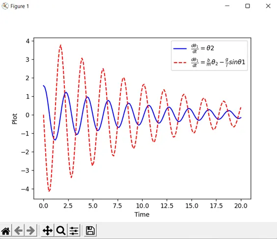

EXPLAINATION-

• To solve ODE second order equation, we break it down into first order ODE equation, as below;
• To solve this, numpy, Scipy, Matplotlib and Math function.
• We calculate ‘dtheta_dt’ with ODE function definition.
• ODE function definition is used to solve initial value problems with variety of properties.
• We used ‘linspace’ command for 150 equal time intervals from 0 to 20 second.
• For creating animation for Simple pendulum, we used ‘for loop’ by defining the distance between the equilibrium position and the extreme position of the pendulum.
• For animation, we used ‘PIL image’ and ‘Golb’ command.
• First, we prepare frames in ‘.png’ format, then convert ‘.png’ into ‘GIF’ file. For this, we used ‘golb’ and ‘natsort’ function.
• We consider a string of length ‘L’ where one end is fixed at co-ordinate (x0 y0) and other end have pendulum /ball shape mass at co-ordinate (x1 y1).
• By using “maker’ command, we create ball size mass.
• After that, we write script for showing simple pendulum in GIF format

ERROR-

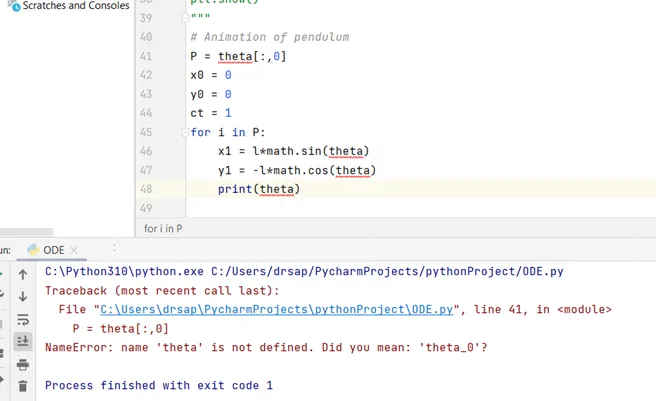
• To overcome this error, we notation ‘i’ instead of ‘theta’.
• We get wrong animation as below.

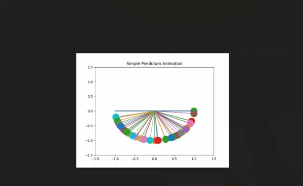
• To overcome this, we used “natsort’ command and we get correct animation.
• Also, write “plt.figure()” at line no 49.

RESULT-

Goggle drive link-

https://drive.google.com/file/d/15en218KBBj5Epki_5LRI53Bzadol-zoH/view?usp=sharing