Week 3 - Solving second order ODEs

TASK: To Write a program in Python that will simulate the pendulum motion

OBJECTIVE:

• To Write a program in Python that will simulate the pendulum motion
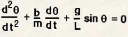
• To write a program that solves the following ODE:

         

PROBLEM STATEMENT:

Using the mass-spring-damper system method, a simple pendulum motion can be described using the equation of motion as:

where,

θ = angular displacement in [radians]

c = damping co-efficient [Ns/m]
m = Mass of the pendulum in [Kg]
l = Length of the string in [meters]
g = acceleration due to gravity in [m/s^2]

As the equation has a highest degree of ‘2’, it is a 2^nd order ODE equation and needs to be converted into 2 simple 1^st order ODEs to sole it using programming. We do that by substituting 1^st order derivative term with a variable ‘θ₂’ such that,

θ = θ₁,

1. ddt">d(θ₁)ddt">/dt= θ₂, and
2. ddt">d(θ2)ddt">/dt =ddt(ddt">d/dt(ddt">d(θ₁)ddt">/dt) = d2dt2">d2(θ₁)/dt2

To solve the ODE in python (integrate) we use ‘odeint’ command from the ‘scipy’ module. Here, we define the ODE as a function, and we solve it for certain initial conditions over an array of ‘t’ time steps which are determined by the program itself. We also have to define the constants/arguments which are a part of the function in specific order.

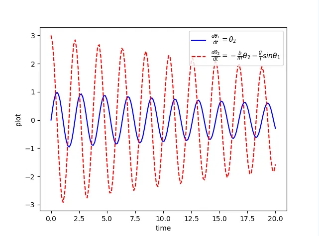
By integrating the ODEs we get an array/list with 2 columns and multiple rows as solution. The 1^st column has the solution of 1^st ODE that is ‘θ₁’ or the angular displacement and the 2^nd column has solution for 2^nd ODE – ‘θ₂’ = θ₁^’ = ‘ω’ or the angular velocity. Using the 1^st solution, θ₁, we can find the co-ordinates of the pendulum for each solution and by assuming the pendulum to be fixed at (0,0) we can plot it as a line for every solution and get the animation.

SOLUTION PROCEDURE:

Step1: Create a Defining Function, which results in displacment and velocity values by using the given ODE Equation.

Step2: Generate various Input Variables such as,

            c = damping co-efficient [Ns/m]
            m = Mass of the pendulum in [Kg]
            l = Length of the string in [meters]
            g = acceleration due to gravity in [m/s^2]

Step3: Then, set an Initail Condition value for angular displacement & velocity as 0 & 3 respectively.Also Generate Time Points.

Step4: Using ODEINT Function to get the values of Final angular displacement & velocity with respect to time.

Step5: To Animate the Simple Pendulum, we have to generate multiple Plots which is used as frames to generate Animation.

Step6: To Plot Multiple Plots, looping Function is Used to Find x1,y1 coordinates Of a pendulum,where other end is fixed(0,0).

Step7: For Ball Structure,we can use Marker size while plotting.

Step8: Finally, Merge all plot frames to Animation.

Program Code:

import math
import matplotlib.pyplot as plt
import numpy as np
from scipy.integrate import odeint


# Function that Returns dtheta/dt
def model(theta,t,b,g,l,m):
	theta1 = theta[0]
	theta2 = theta[1]
	dtheta1_dt = theta2
	dtheta2_dt = -(b/m)*theta2 - (g/l)*math.sin(theta1)
	dtheta_dt = [dtheta1_dt,dtheta2_dt]
	return dtheta_dt
	return theta1

# inputs 
b=0.05
g=9.81
l=1
m=1

# initial Conditions
theta_0 = [0,3]

# timepoints
t=np.linspace(0,20,150)

#solve ODE
theta = odeint(model,theta_0,t,args=(b,g,l,m))

angular_displacement = []
angular_velocity = []



# Plot Results


plt.plot(t,theta[:,0],'b-',label=r'$\frac{d\theta_1}{dt}=\theta_2 $')
plt.plot(t,theta[:,1],'r--',label=r'$\frac{d\theta_2}{dt}= -\frac{b}{m}\theta_2 - \frac{g}{l} sin\theta_1$')
plt.ylabel('plot')
plt.xlabel('time')
plt.legend(loc='best')
plt.show()

for j in range(0,len(theta)):
	displacement = theta[j,0]
	angular_displacement.append(displacement)

	velocity = theta[j,1]
	angular_velocity.append(velocity)
# initial POints
x0=0
y0=0
ct=1
for i in range(0,len(t)):
	theta = angular_displacement[i]
	x1 = 1*math.sin(theta)
	y1 = -1*math.cos(theta)
	filename=str(ct)+'.png'
	ct=ct+1



# animation plot frames
	plt.figure()
	plt.plot([-1,1],[0,0],color="red")
	plt.plot([x0,x1],[y0,y1])
	plt.plot(x1,y1,marker='o',markerfacecolor='g',markeredgecolor='k',markersize=16)
	plt.xlim([-3,3])
	plt.ylim([-3,3])
	plt.title('Animation of simple pendulum motion',fontsize=20,fontweight='bold')
	plt.savefig(filename)

Displacement and velocity Plots: 

Animation of a simple pendulum:

https://youtu.be/c_I12G4TSnk

Conclusion:

 Thus,a program to simulate the pendulum motion is created.