Challenge

Project 2

Project 2:
Project 2 deals with the development of a forward energy-based fuel consumption model of a P1 hybrid vehicle. This model is based on the conventional vehicle model from Project 1:

% MATLAB SCRIPTS:

Project2_InitFile.m:

%%%%%%%%%%%%%%%%%%%%%%%%%%%%%%%%%%%%%%%%%%%%%%%%%%%%%%%%%%%%%%%%%%%%%
%% Skill-Lync -> Hybrid Drives Development
% Project 1 - Conventional Vehicle Model
% By - Ullekh Gambhira
% Description:
%% Initialization File
% Initialization file for loading the variables for the Conventional vehicle simulation model
%% Vehicle Parameters
M = 1500; % Vehicle weight [kg]
Cr = 0.015; % Rolling resistance coefficient
Rw = 0.35; % Rolling radius [m]
Cd = 0.33; % Drag coefficient
Af = 2; % Frontal area [m2]
rhoa = 1.225; % Air density [kg/m3]
Vwind = 0; % Wind velocity [kmph]
g = 9.81; % Gravitational acceleration [m/s2]
theta = 0; % Slope [deg]
myu_road_tire = 1; % Coefficient of friction between tire - road interface
%% Powertrain Parameters
FDR = 3.73; % Final Drive Ratio / Diff Ratio
DiffEff = 0.99; % Differential efficiency (assumed independent of operating conditions)
NumGear = 4; % Number of gears in transmission
TransGear = [1:NumGear]; % Transmission Gears
TransRatio = [3.06, 1.62, 1, 0.7]; % Corresponding Transmission ratios
TransEff = 0.90; % Transmission efficiency (assumed independent of operating conditions)
TC_SR = [0, .5, .6, .7, .8, .87, .92, .94, .96, .97, 1]; % Torque Converter Speed Ratio (Matlab default) -> TurbSpd/PumpSpd
TC_TR = [2.232, 1.5462, 1.4058, 1.2746, 1.1528, 1.0732, 1.0192, 1, 1, 1, 1]; % Torque Converter Torque Ratio (Matlab default) -> TurbTrq/PumpTrq
TC_Cf = 1e-4 * [.72558, .66322, .63463, .59042, .51331, .4144, .29287, .22444, .12186, .04386, 0]; % Torque Converter Capacity Factor (Matlab default) -> PumpTrq/PumpSpd^2 [Nm/rpm^2]
load Engine_data_1_9L_Saturn_95kW
load Trans_Shift_map
load EM_Honda_Insight_10kW
load ESS_NiMH6
ESS_init_soc = 0.8;
ESS_soc_max = 0.9;
ESS_soc_min = 0.6;
%% Driver Parameters
Kp = 10; % P gain for driver PI model
Ki = 1; % I gain for driver PI model
Drive_Cycle_Select = 2; % Drive cycle selection
% Drive cycle values in m/s
if Drive_Cycle_Select == 1
load UDDS;
elseif Drive_Cycle_Select == 2
load HWFET;
elseif Drive_Cycle_Select == 3
load FTP;
elseif Drive_Cycle_Select == 4
load US06;
elseif Drive_Cycle_Select == 5
load NEDC;
elseif Drive_Cycle_Select == 6
load WLTP;
end
time_end = cyc_time(end);
vel_end = cyc_vel(end);
Simulink Model Results:

Forward Model:-

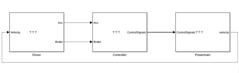
It also known as dynamic simulation. Dynamic models are used for detailed simulations. In this model force/torque/power is the input and the vehicle state variable velocity and acceleration are outputs. The models and simulatios are more realistic due to phhysical casualty hence appropriate for control development. There is feedback loop to meet the desired vehicle state. It is mainly used to simulate a vehicle on a driving cycle to analyse the dynamic behaviour of the system helps significantly in control development.

1) Driver:

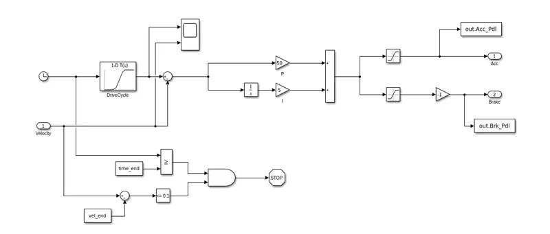
It is modeled using a ‘Driver’ block, which is a basic PI controller that generates accelerator and brake pedal outputs to match the desired and actual vehicle speeds. In this we use drive cycles fro the based on these results of fuel consumption and emissions the vehicle gets certified and it also forms a basis of uniform asessment. It is based on time, velocity then its all integrate and creates output accelration pedal and brake pedal.

2) Controller:

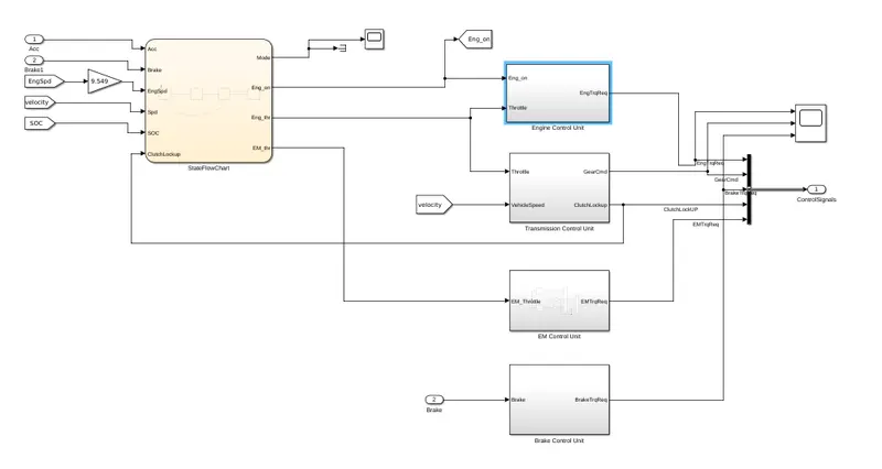
The ‘Controller’ block is the brains of the vehicle, representing the electronic controls units. It is based on the driver inputs, it generates desired engine torque, desired transmission gear and desired brake torque. These inputs are fed to the ‘Powertrain’ block which represents the drivetrain of the vehicle.

i) EM CONTROL UNIT:

3) POWERTRAIN:
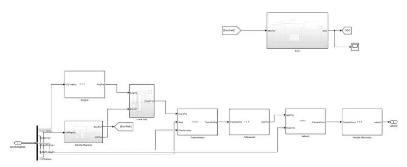
The powertrain encompasses every component that converts the engine's power into movement. This includes the engine, transmission, the driveshaft, differentials, axles; basically anything from the engine through to the rotating wheels.
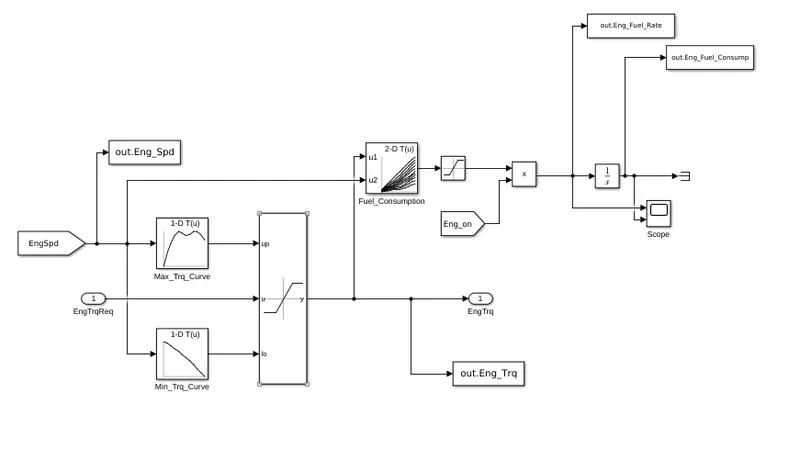
I) ENGINE:
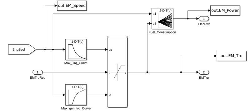
II) ELECTRIC MOTOR:
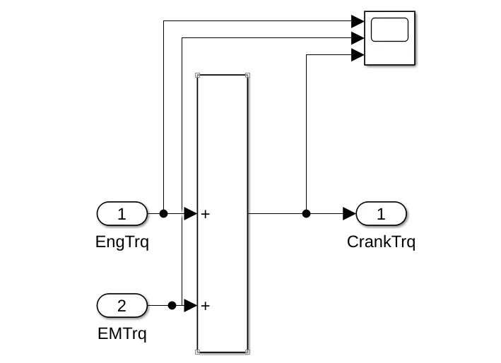
III) CRANK HUB:
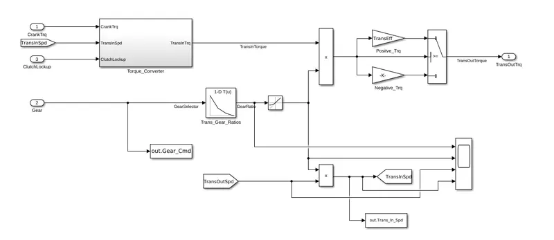
IV) TRANSMISSION:
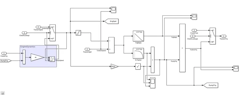
A) TORQUE CONVERTER:
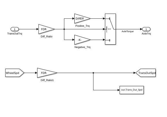
V) DIFFERENTIAL:
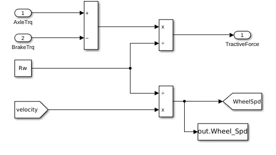
VI) WHEELS:
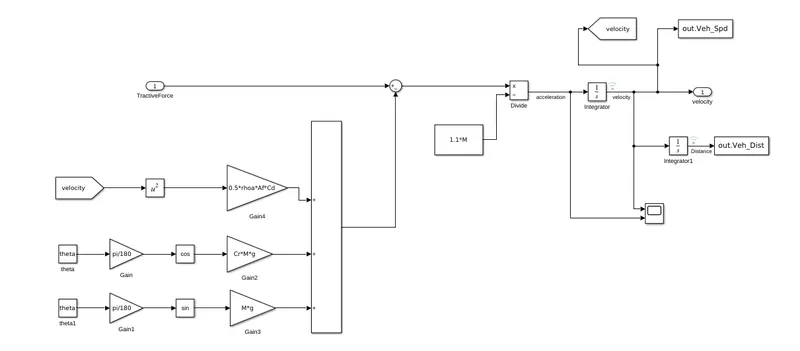
VII) VEHICLE DYNAMICS:

In this takes tractive force and road load. It is dictates vehicle speed based on tractive force and road load.

the dynamic equation for calculating road load is

MeqdVveh/dt=ηtλtot/Rw*Tm-(1/2p⋅A⋅Cd⋅(Vveh+Vw∈d)2+Cr⋅M⋅g⋅cos(θ)+M⋅g⋅sin(θ))

where,

p = air density [kg/m^3]

A = Frontal area [m^2]

Cd = drag Coefficiend

Vveh = velocity of vehicle [m/s^2]

Vwind = velocity of wind [m/s^2]

Cr = rolling resistance coefficient

M = mass in [Kg]

g = gravity.

Then we calculate and integrate then we meet acceleration of vehicle and velocity of vehicle it mean vehicle distance and vehicle speed.

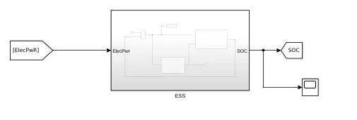
BATTERY ESS SYSTEM:

% MATLAB SCRIPTS:

Project2_ProcessingFile.m:

%%%%%%%%%%%%%%%%%%%%%%%%%%%%%%%%%%%%%%%%%%%%%%%%%%%%%%%%%%%%%%%%%%%%%
%% Skill-Lync -> Hybrid Drives DevelopmentS
% Project 1 - Conventional Vehicle Model
% By - Ayyappan G
% Description:
% The following file is to used with the Initialization file and Simulink
% results for post-processing of the data.
% The file is incomplete, has some examples of how the data is imported
% into a readable format, data analysis and plotting examples.
% Based on the project task, use commands in a similar format as given
% below, to analyse the data and generate required plots.
% You can change variable names if desired
%% Post-Processing File
% File for post-processing the Conventional vehicle simulation model data
%% Renaming variables
Time = out.tout;
Acc_Pdl = out.Acc_Pdl; % Accelerator pedal [%]
Brk_Pdl = out.Brk_Pdl; % Brake pedal [%]
Gear_Cmd = out.Gear_Cmd; % Transmission gear
Trans_In_Spd = out.Trans_In_Spd*30/pi; % Transmission input speed [rpm]
Trans_Out_Spd = out.Trans_Out_Spd*30/pi;% Transmission output speed [rpm]
Eng_Trq = out.Eng_Trq; % Engine brake torque [Nm]
Eng_Spd = out.Eng_Spd*30/pi; % Engine speed [rpm]
Eng_Fuel_Consump = out.Eng_Fuel_Consump; % Engine fuel consumption [g]
Veh_Dist = out.Veh_Dist/1000; % Distance traveled by vehicle [km]
Veh_Spd = out.Veh_Spd*18/5; % Vehicle speed [kmph]
Wheel_Spd=out.Wheel_Spd;
Eng_Fuel_Rate=out.Eng_Fuel_Rate;
EM_Speed=out.EM_Speed;
EM_Power=out.EM_Power;
EM_Trq=out.EM_Trq;
I_pack=out.I_pack;
TerminalVoltage=out.TerminalVoltage;
SOC=out.SOC;
%% Data Analysis
Eng_Pwr = Eng_Spd*pi/30*Eng_Trq/1000; % Engine brake power [kW]
rho_petrol = 0.7197; % Density of petrol [kg/L]
%% Plotting vehicle characteristics time trace to Engine speed, Engine Torque, Engine Power,
% And Engine fuel rate, Engine fuel consumption
% Data conversion from Double Timeseries
Eng_spd = Eng_Spd.Data(:,1); % engine speed
Eng_trq = Eng_Trq.Data(:,1); % engine torque
Eng_pwr = Eng_Pwr.Data(:,1); % engine power
Eng_fuel_rate = Eng_Fuel_Rate.Data(:,1); % engine fuel rate
Eng_fuel_consumption = Eng_Fuel_Consump.Data(:,1); % engine fuel consumption
Veh_dist = Veh_Dist.Data(:,1); % vehicle distance
Veh_spd = Veh_Spd.Data(:,1); % vehicle speed
Wheel_spd = Wheel_Spd.Data(:,1);
Eng_pwr = Eng_Pwr.Data(:,1);
EM_speed = EM_Speed.Data(:,1);
EM_trq = EM_Trq.Data(:,1);
EM_power = EM_Power.Data(:,1);
Terminalvoltage = TerminalVoltage.Data(:,1);
%I_Pack=I.pack(:,1);
soc=SOC(:,1);
% Plotting Time Vs'Trans Input','Trans Output','Wheel Speed'
figure(1)
hold on
grid on
plot(Time, Trans_In_Spd, 'linewidth', 1, 'Color', 'blue');
plot(Time, Trans_Out_Spd, 'linewidth', 1, 'Color', 'green');
plot(Time, Wheel_spd, 'linewidth',1, 'color', 'black')
ylabel('Speed [rpm]')
xlabel('Timem [s]')
xlim([0, Time(end)]);
ylim([0, 3000]);
legend('Trans Input','Trans Output','Wheel Speed');
%subplots for Torque,Power,Fuel Rate,Fuel Consumption
figure(2)
subplot(2,2,1)
plot(Time,Eng_trq,'linewidth',1,'color','black')
xlabel('Time [s]')
ylabel('Torque [Nm]')
legend('Engine Torque')
grid on
subplot(2,2,2)
plot(Time,Eng_pwr,'linewidth',1,'color','blue')
xlabel('Time [s]')
ylabel('Power [KW]')
legend('Engine Power')
grid on
subplot(2,2,3)
plot(Time,Eng_fuel_rate,'linewidth',1,'color','red')
xlabel('Time [s]')
ylabel('Fuel Rate [%]')
legend('Engine Fuel Rate')
grid on
subplot(2,2,4)
plot(Time,Eng_fuel_consumption,'linewidth',1,'color','green')
xlabel('Time [s]')
ylabel('Fuel Consumption')
legend('Engine Fuel Consumption')
grid on
%% Plotting vehicle characteristics time trace
figure(3)
subplot(3,2,1)
hold on
grid on
plot(Time, Acc_Pdl, 'linewidth', 1, 'Color', 'black');
plot(Time, Brk_Pdl, 'linewidth', 1, 'Color', 'red');
ylabel('Pedal [%]')
xlim([0, Time(end)]);
legend('Accel','Brake');
subplot(3,2,2)
hold on
grid on
plot(Time, Trans_In_Spd, 'linewidth', 1, 'Color', 'black');
plot(Time, Trans_Out_Spd, 'linewidth', 1, 'Color', 'red');
ylabel('Speed [rpm]')
xlim([0, Time(end)]);
ylim([0, 6000]);
legend('Trans Input','Trans Output');
subplot(3,2,3)
hold on
grid on
plot(Time, Gear_Cmd, 'linewidth', 1, 'Color', 'black');
xlim([0, Time(end)]);
xlabel('Time [s]');
ylabel('Gear');
subplot(3,2,4)
hold on
grid on
plot(Time, Wheel_spd, 'linewidth', 1, 'Color', 'black');
plot(Time, Veh_spd, 'linewidth', 1, 'Color', 'red');
ylabel('Speed [rpm]')
xlim([0, Time(end)]);
legend('Desired Speed','Actual Speed');
subplot(3,2,5)
hold on
grid on
plot(Time, Veh_dist, 'linewidth', 1, 'Color', 'blue');
xlim([0, Time(end)]);
xlabel('Time [s]');
ylabel('Distance');
%% Plotting engine operating points on engine fuel map
figure('Name','Engine Operating Points');
hold on
grid on
title('Engine Operating Points','fontsize',12);
p1=plot(Eng_map_spd*30/pi,Eng_max_trq,'linewidth',2,'color','r');
p2=line([Eng_map_spd(end)*30/pi Eng_map_spd(end)*30/pi],[0 Eng_max_trq(end)]);
set(p2,'linewidth',1,'linestyle','--','color','k');
p3=line([Eng_map_spd(1)*30/pi Eng_map_spd(1)*30/pi],[0 Eng_max_trq(1)]);
set(p3,'linewidth',1,'linestyle','--','color','k');
[c,h] = contour(Eng_map_spd'*30/pi,Eng_map_trq,Eng_fuel_map');
clabel(c,h);
xlabel('Engine Speed [rpm]');
ylabel('Engine Torque [Nm]');
title('Engine Fuel Consumption Map [g/s]');
p4 = plot(Eng_spd,Eng_trq,'.','color','k');
legend([p1 p4],{'Max Curve','Operating Points'});
axis([Eng_map_spd(1)*30/pi Eng_map_spd(end)*30/pi 0 Eng_map_trq(end)]);
%%Plot motor speed, torque, motor input power using subplots:
figure(5)
subplot(3,1,1)
plot(Time,EM_speed,'linewidth',1,'color','black')
xlabel('Time [s]')
ylabel('Motor speed Rpm')
legend('Motor speed')
grid on
subplot(3,1,2)
plot(Time,EM_trq,'linewidth',1,'color','blue')
xlabel('Time [s]')
ylabel('Motor Torque Nm')
legend('Motor Torque')
grid on
subplot(3,1,3)
plot(Time,Eng_pwr,'linewidth',1,'color','red')
xlabel('Time [s]')
ylabel('Motor Input Power')
legend('Motor Input Power')
grid on
%% Plot pack voltage, current and SoC using subplots:
figure(6)
subplot(3,1,1)
plot(Time,Terminalvoltage,'linewidth',1,'color','black')
xlabel('Time [s]')
ylabel('Voltage')
legend('Voltage')
grid on
subplot(3,1,2)
plot(Time,I_pack,'linewidth',1,'color','blue')
xlabel('Time [s]')
ylabel('Current')
legend('Current')
grid on
subplot(3,1,3)
plot(Time,soc,'linewidth',1,'color','red')
xlabel('Time [s]')
ylabel('soc')
legend('soc')
grid on
%% Plotting engine operating points on engine fuel map
figure('Name','Motor Operating Points');
hold on
grid on
%%Plot the motor operating points on the motor input power map, with the motor max motoring and generating torque curves:
title('Motor Operating Points','fontsize',12);
p1=plot(EM_map_spd*30/pi,EM_max_trq,'linewidth',2,'color','r');
p2=line([EM_map_spd(end)*30/pi EM_map_spd(end)*30/pi],[0 EM_max_trq(end)]);
set(p2,'linewidth',1,'linestyle','--','color','k');
p3=line([EM_map_spd(1)*30/pi EM_map_spd(1)*30/pi],[0 EM_max_trq(1)]);
set(p3,'linewidth',1,'linestyle','--','color','k');
xlabel('Motor Speed [rpm]');
ylabel('Motor Torque [Nm]');
title('Motor Operating Points');
p4 = plot(EM_speed,EM_trq,'.','color','k');
legend([p1 p4],{'Max Curve','Operating Points'});
axis([EM_map_spd(1)*30/pi EM_map_spd(end)*30/pi 0 EM_map_trq(end)]);
%% Data Analysis
kmpl = Veh_dist(end)/(Eng_fuel_consumption(end)/1000/rho_petrol); % Fuel economy [kmpl]
Results:
a)Tabulate the fuel economy numbers (kmpl) for UDDS and HWFET cycle. Compare these numbers with the baseline numbers for conventional vehicle model from Project 1:
Project 2 Result:
FUEL ECONOMY RATE(KMPL)
S.NO DRIVE CYCLES kmpl
1 UDDS DRIVE CYCLE 16.195
2 HWFET DRIVE CYCLE 17.53

Project 1 Result:

FUEL ECONOMY RATE(KMPL)
S.NO DRIVE CYCLES kmpl
1 UDDS DRIVE CYCLE 13.63
2 HWFET DRIVE CYCLE 16.307
Plot Results for UDDS Drive Cycle:
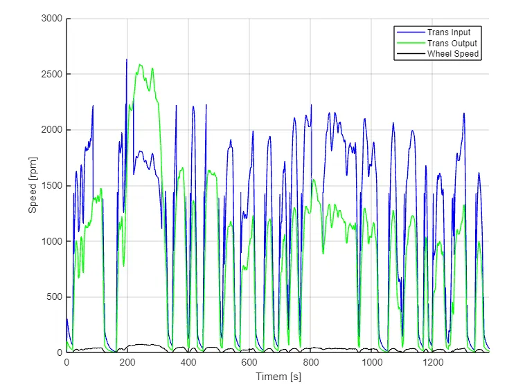
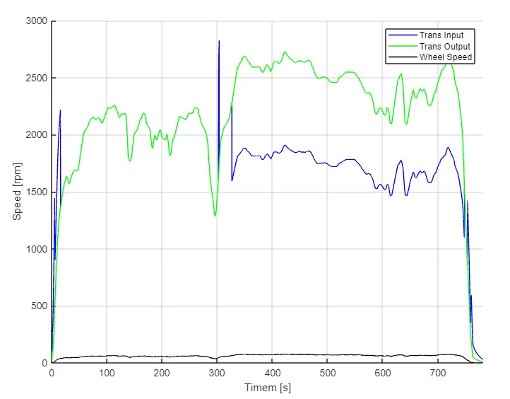
1)Plot the time trace for engine, transmission input, transmission output and wheel speed
Many ups and Down in Speeds because Udds In drive Cycle Run in Traffic Area,not Like Hwfet.
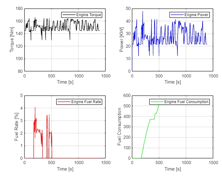
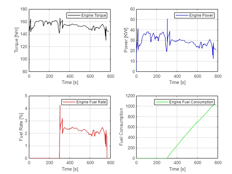
2)Plot engine torque, engine power, fuel rate and fuel consumption using subplots
By comparing torque ,power fuel rate there are several ups and downs due to inconsistant speed rate more stops are applied on traffic city sides and also fuel consumption is not more steady as compared to hwfet.
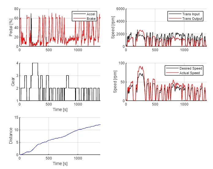
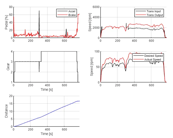
3) Plot accelerator and brake pedal, gear command, vehicle desired and actual speed, vehicle distance using subplots.

In this Plot it is Clear that accelertion pedal is high it is controlled by brake pedal to some extent.

then desired speed from the wheel is reduced here after some losses happened in the vehicle dynamics.

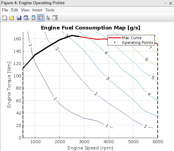
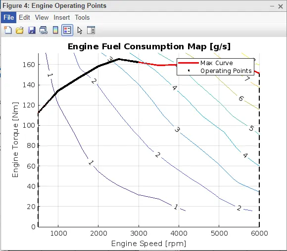
4) Plot the engine operating points on the engine fuel map
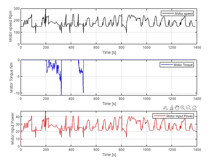
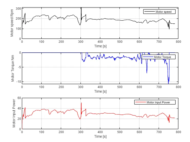
5) Plot motor speed, torque, motor input power using subplots
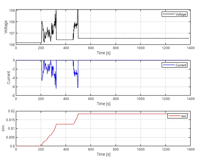
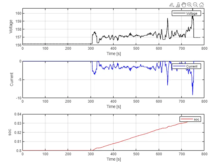
6)Plot pack voltage, current and SoC using subplots
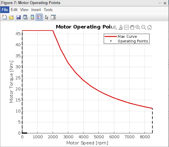
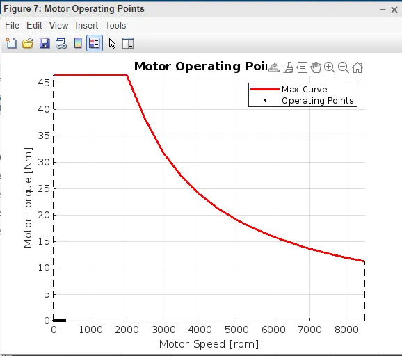
7)Plot the motor operating points on the motor input power map, with the motor max motoring and generating torque curves:
Plot Results fow HWFET Drive Cycle:
1)Plot the time trace for engine, transmission input, transmission output and wheel speed
Not Many ups and Downs in Speeds As in Udds because HWFET runs in Highways.
2)Plot engine torque, engine power, fuel rate and fuel consumption using subplots

By comparing torque ,power fuel rate there are more upside due to consistant speed rate and less stops are applied on Highway and also fuel consumption is more steady as compared to UDDS.

3) Plot accelerator and brake pedal, gear command, vehicle desired and actual speed, vehicle distance using subplots.

In this Plot it is Clear that accelertion pedal is too high it is controlled by brake pedal to some extent.

then desired speed from the wheel is incresed here after some losses happened also in the vehicle dynamics.

4) Plot the engine operating points on the engine fuel map
5) Plot motor speed, torque, motor input power using subplots
6)Plot pack voltage, current and SoC using subplots
7)Plot the motor operating points on the motor input power map, with the motor max motoring and generating torque curves:
CONCLUSION:
Hence, We Concluded here With Various Plots of Vehicle Characteristics.
Also Comparing the Kmpl of Both Conventional and Hybrid Vehicles:
Hybrid:
FUEL ECONOMY RATE(KMPL)
S.NO DRIVE CYCLES kmpl
1 UDDS DRIVE CYCLE 16.195
2 HWFET DRIVE CYCLE 17.53

Conventional:

FUEL ECONOMY RATE(KMPL)
S.NO DRIVE CYCLES kmpl
1 UDDS DRIVE CYCLE 13.63
2 HWFET DRIVE CYCLE 16.307
Your portfolio, next

Ship work like this
in your own course.

Talk to a career counsellor

Free 20-minute call. We'll map the right course to where you want to work.

By submitting you agree to our Terms and Privacy Policy.