Week 3 - Solving second order ODEs
Aim- To write a program that solves the ODE. This ODE represents the equation of motion of a simple pendulum with damping. And make animation for simple pendulum.
Theory-In mathematics, an ordinary differential equation is a differential equation containing one or more functions of one independent variable and the derivatives of those functions. The term ordinary is used in contrast with the term partial differential equation which may be with respect to more than one independent variable.
In mathematics, an ordinary differential equation is a differential equation containing one or more functions of one independent variable and the derivatives of those functions. The term ordinary is used in contrast with the term partial differential equation which may be with respect to more than one independent variable.
In general, solving an ODE is more complicated than simple integration. Even so, the basic principle is always integration, as we need to go from derivative to function. Usually, the difficult part is determining what integration we need to do.
here,we use ODE 45 which is based on the Runge kutta method,which is 4th order runge kuta method
ode-45, used to solve higher order differential equations because its solution or outputs not vary rapidly means its solutions are very smooth.
Equations/formulaes-
in this project problem is given of 2nd order diff.eq. as, (d^2theta/dt)+b/m(d theta/dt)+g/l*sin theta=0
where, theta=theta1-displacement, dtheta/dt =theta2 -velocity,
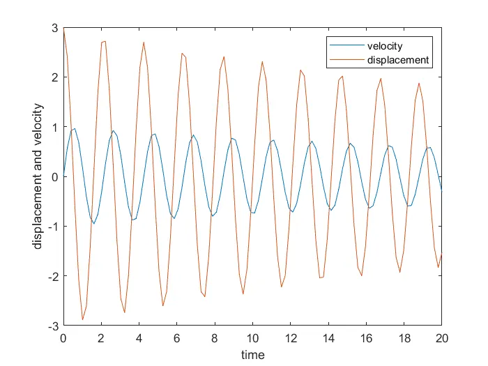
so here weare finfding the value of velocity and displacemet with the rate which is change with respect to time .
where,b= damping coefficient, m=mass of bob, l=length df string, g= acc.due to gravity,
{dtheata/dt=dtheta1/dt=theta2};-------1
{d^2theta/dt^2= (d^2theta1/dt^2) =d/dt(dtheta1/dt)= d/dt (theta2)---------2
we have 2d order ode,
{d^2theta/dt^2 +b/m(dtheta/dt)+g/l(sin theta)};
by simplifying it, {d^2theta1)/dt +b/m(dthet1/dt) +g/l(sin theta1)=0};
by eq 1and 2,
{dtheta2/dt+b/m(theta2)+g/l(sin theta1)}=0
{dtheta^2/dt=-b/m(theta2)-g/l (sintheta1)};
so we convert 2nd order ode into two 1st order ode,
as,follow
dtheta^2/dt=-b/m(theta2)-gl(sin theta1)--------3
dtheta1/dt=theta2-------4
now by using eq 3 and 4 animate a simple pendulum.
matlab-code
% function call for the ode challange

function [dtheta_dt]= ode_fun(t,theta,b,g,l,m)

theta1=theta(1);
theta2=theta(2);

% BY SOLVING ON BOOK YOU KNOW WE SEPRATE 1ST ORDER AND 2ND ORDER ODE
% MEANS dtheta1_dt is 1st order ode $ dtheta2_dt is 2nd order ode

dtheta1_dt=theta2;
dtheta2_dt= -(b/m)*theta2-(g/l)*sin(theta1);
dtheta_dt=[dtheta1_dt; dtheta2_dt];
end
main code-
%CODE FOR SOLVING 2ND ORDER ODE EQUATION AND ANIMATING PENDULAM

%inputs for pendulam in 2nd order ODE
b=0.05;  % damping coefficent

g=9.81;  % acc. due to garvity

l=1;     % length of string

m=1;     % mass of bob (pendulam)

%intial condition, theta_0 = [displacement;velocity]

%inial displacement=0 and intial velocity=3

 theta_0=[0;3]; % - is due to column matrix

% time points
t_span = linspace(0,20,100);

% solve ODE  by (function call)
[t,results] = ode45(@(t,theta) ode_fun(t,theta,b,g,l,m),t_span,theta_0);

%plotting displacement and velocity with time
figure(1)
plot(t,results(:,1))
hold on
plot(t,results(:,2))
xlabel('time')
ylabel('displacement and velocity')
legend('velocity','displacement')


% animation for pendulam

new_theta=(results(:,1))
ct=1
figure(2)
for i= 1:length(new_theta)

ta=new_theta(i)

%co-ordinates
%fix point of pendulam or the bob at top
x0= 0
y0= 0

% end co-ordinates for the bob
x1=l*sin(ta)
y1=-l*cos(ta)

%plotting for pendulam/bob

%for horizontal line
plot([-1 1],[0 0], 'LineWidth',4,'Color','c')
hold on

%piovet
plot([0 0],[0 0], 'o','MarkerFaceColor','k','MarkerSize',8)

%string
plot([x0 x1],[y0 y1],'LineWidth',3,'Color','m')

% creat bob/pendulam
plot(x1,y1, 'o','MarkerFaceColor','g','MarkerSize',35)

hold off % to remove previous position for new

axis([-1.5 1.5 -1.5 0.5])

pause(0.03)
M(ct)= getframe(gcf)
ct=ct+1;
end

movie(M)
Videofile=VideoWriter('simple-pendulum2.avi','Uncompressed AVI')
open(Videofile)
writeVideo(Videofile,M)
close(Videofile)
explanation- first we have to make function go this challange
save this file as a name of your funcion
function should includde- the given inputs i.e b,g,l,m,t and theta
which is nothing but the
b- damping coefficient -nm/s
g- acc.due to gravity- m/s^2
l-length of the string- m
m- mass of the bob -kg
t- time span
theta- included the value of velocity and displacement
now in the main code , put the given values of inputs like b,g,l,m and t
gives the intial condition of displacement and velocity as theta_0
initial displacement must be 0 and velocity is 3 as mentioned in challange
create a range for time using the linspace command
plot disp.and velocity with respect to time
now for the animation of the pendulum,use for loop and ct=1
now plot the co-ordinates at top and bottom for the pendulum as, x0y0 and x1y1
now plot the horizontal lline, piovet,string, and create bob/pendulum
now create the axis for the animation.
now at last create movie for the animation of pendulum by using commands like,
getframe, videowriter,videofile,writevideo, and close at the end by usinfg close command
following is the graph for the displacement and velocity with respect to time.
link for animation of the pendulum as follows,
https://drive.google.com/file/d/1qSDY6_cpR4N83zGlJ-asJXDuPAkxOlhh/view?usp=sharing