Project 2 - Rankine cycle Simulator
Q-Understand the concept of Rankine cycle by referring to standard thermal engineering text book.
- Create a Rankine Cycle Simulator using OCTAVE/MATLAB.
- Your code should calculate the state points of the Rankine Cycle (any type of your choice) based on user inputs.
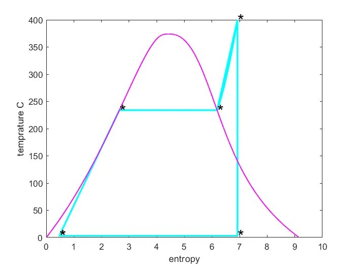
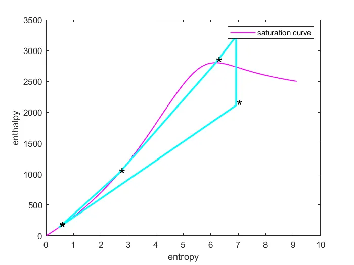
- Then, plot the corresponding T-s and h-s plots for the given set of inputs. Title and axes labels are a must, while legends could be used if necessary.
- The presentation of your code will be taken into consideration while grading. Labelling sections of your code using comments is appreciated.
- Attach a report explaining the working of a rankine cycle simulator and also the research done by you.
AIM- Calculate the state points of the Rankine Cycle using given input.
Plot the corresponding T-s and h-s plots for the given set of inputs.
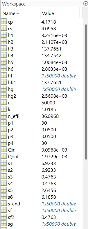
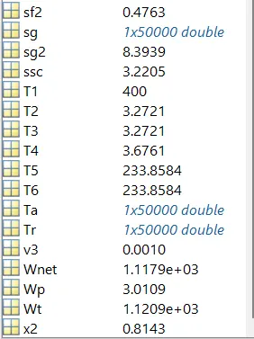
All outputs are shown in command window through coding.
THEORY- The Rankine cycle is an idealized thermodynamic cycle of a constant pressure heat engine that converts part of heat into mechanical work. In this cycle, the heat is supplied externally to a closed loop, which usually uses water (in a liquid and vapor phase) as the working fluid. In contrast to the Brayton cycle, the working fluid in the Rankine cycle undergo the phase change from a liquid to vapor phase and vice versa.
While many substances could be used as the working fluid in the Rankine cycle (inorganic or even organic), water is usually the fluid of choice due to its favorable properties, such as its non-toxic and unreactive chemistry, abundance, and low cost, as well as its thermodynamic properties.
Moreover , it has a very high heat of vaporization, making it an effective coolant and medium in thermal power plants and other energy industries. In the case of the Rankine cycle, the Ideal Gas Law almost cannot be used (steam does not follow pV=nRT). Therefore all important parameters of water and steam are tabulated in so-called''Steam Tables''.
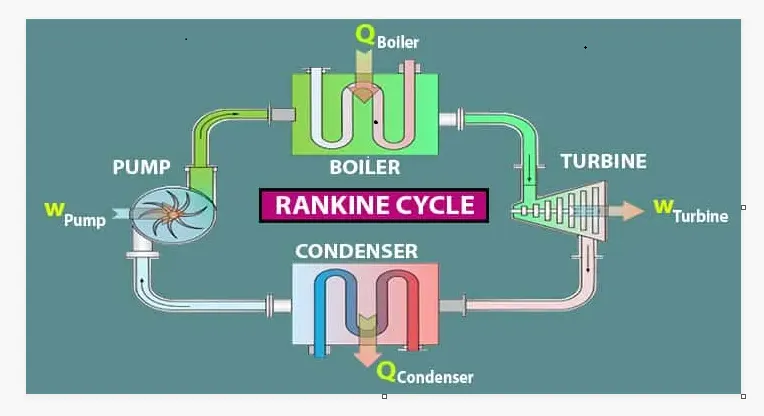
There are four main components Rankine cycle system,
1) Pump
2) Boiler
3) Turbine
4) Condenser
And four important processes are,
1-2 Isentropic compression in a pump
2-3 Constant pressure heat addition in a boiler
3-4 Isentropic expansion in a turbine
4-1 Constant pressure heat rejection in a condenser
Component 1 -pump
Process 1-2 indicates pump in Rankine cycle
Work done incurs in the system
Pressure increases in this stage.
Component 2 -boiler
Point 2-3 represent the boiler in the cycle
Heat is added in the high-pressure fluid by the boiler
Temperature increases upto the boiling point
Water changes into vapor as its phase changes.
Component 3 -turbine
Point 3-4 indicates the turbine in the cycle
Expansion happens in the turbine
Component 4 -condenser
Point 4-1 indicates the condenser
Waste heat is removed from the condenser with
With the help of the condensation process
Process 1–2: The working fluid is pumped from low to high pressure. As the fluid is a liquid at this stage, the pump requires little input energy.
Process 2–3: The high-pressure liquid enters a boiler, where it is heated at constant pressure by an external heat source to become a dry saturated vapor. The input energy required can be easily calculated graphically, using an enthalpy–entropy chart (h–s chart, or Mollier diagram), or numerically, using steam tables.
Process 3–4: The dry saturated vapor expands through a turbine, generating power. This decreases the temperature and pressure of the vapor, and some condensation may occur. The output in this process can be easily calculated using the chart or tables noted above.
Process 4–1: The wet vapor then enters a condenser, where it is condensed at a constant pressure to become a saturated liquid.
important formulas-
Thermal efficiency, η = Wturbine – Wpump / Qboiler
Where,
W turbine- is the work output
W pump -is work input
Q boiler is the heat supplied.
nth= {(Wnet/Qin)*100};
h1: Enthalpy at point 1
h2 :Enthalpy at point 2
h3 :Enthalpy at point 3
h4: Enthalpy at point 4
clear all
close all
clc

disp("RANKIN CYCLE")

disp('1-2 IS CONSTANT PRESSURE HEAT ADDITION PROCESS AT BOILER')
disp('2-3 IS ICENTROPIC PROCESS AT TURBINE')
disp('3-4 IS CONSTANT PRESSURE HEAT REJECION PROCESS AT CONDENSER')
disp('4-1 IS ICENTROPIC PROCESS AT PUMP')

% INPUT AT STATE 1( TURBINE INLET)
p1=30; %PRESSURE IN BAR(AT TURBINE INLET)
T1=400; %TEMPRATURE IN DEGREE.C (AT TURBINE INLET)
p2=0.05; %PRESSURE IN BAR(AT CONDENSER INLET)

% THERE IS SUPERHEATED CONDITION AT GIVEN TEMP.400.C AT PRESURE 30 BAR

h1=XSteam('h_pT', p1,T1); % ENTHALPLY AT STATE 1 IN KJ/Kg
s1=XSteam('s_pT',p1,T1); % ENTROPY AT STATE 1 IN KJ/Kg K


% STATE 2 (CONDENSER INLET)
% h2= hf2 + (x2*(hg2-hf2));
s2=s1; %( DUE TO ISENTROPIC EXAPANSION)
hf2= XSteam('hl_p',p2); %saturated fluid enthalpy
hg2= XSteam('hv_p',p2); %saturated vapour enthalpy
sf2= XSteam('sl_p',p2); %saturated fluid entropy
sg2= XSteam('sv_p',p2); %saturated vapour entropy
x2=(s2-sf2)/(sg2-sf2);  %Dry ness fractioin
T2=XSteam('T_ps',s2,p2);
h2=hf2 + (x2*(hg2-hf2));


%STATE 3(PUMP INLET)
%h3=hf2=hf3=hl_p at p2 ,, p3=p2 i.e
p3=p2;
h3=XSteam('hl_p',p3);
s3=XSteam('sl_p',p3);
T3=T2;


%STATE 4 (BOILER INLET)
p4=p1;
s4=s3;
v3=XSteam('vl_p',p3);%
% work done by pump
Wp=v3*(p4-p3)*100
h4=h3-Wp;

cp=XSteam('cp_ps',p4,s4); % heat capacity at constant pressure
cv=XSteam('cv_ps',p4,s4); % heat capacity at constant volume

k=cp/cv

T4=T3/((p3/p4)^((k-1)/k));

%STATE 5-6
h5=XSteam('hl_p',p1);
s5=XSteam('sl_p',p1);
T5=XSteam('tsat_p',p1);

h6=XSteam('hv_p',p1);
s6=XSteam('sv_p',p1);
T6=T5;

%-----------------------------------------------%
% PLOTTING T-S DIAGRAM
Tr= linspace(T1,T5,50000) % (T5=T6)
for i= 1:length(Tr)

    s_end(i) = XSteam('s_pt',p1,Tr(i));% i.e s_end =s1(bcz of loop)
end
plot([s1,s2,s3,s4,s5,s6,s_end],[T1,T2,T3,T4,T5,T6,Tr],'linewidth',2,'Color','c')
hold on

% plotting saturation curve in t-s diagram
Ta=linspace(1,400,50000)
  for i=1:length(Ta)
      sf(i)=XSteam('sl_t',Ta(i));
      sg(i)=XSteam('sv_t',Ta(i));
     hf(i)=XSteam('hl_t',Ta(i));
     hg(i)=XSteam('hv_t',Ta(i));


  end
  figure(1)

  plot(sf,Ta,'Color','m','LineWidth',1);
  plot(sg,Ta,'Color','m','LineWidth',1);


hold on


text(s1,T1,'*','FontSize',20)
text(s2,T2,'*','FontSize',20)
text(s3,T3,'*','FontSize',20)
text(s4,T4,'*','FontSize',20)
text(s5,T5,'*','FontSize',20)
text(s6,T6,'*','FontSize',20)
xlabel('entropy')
ylabel('temprature C')


%--------------------------------------%
 figure(2)


% plotting saturation curve in h-s diagram
% sf,hf - are the specific entropy and specfic enthalpy for fluid
% sg,hg - are the specific entropy and specfic enthalpy for vapour

plot(sf,hf,sg,hg,'color','m','LineWidth',1);


hold on

% POTTING H-S DIAGRAM
plot([s1,s2,s3,s4,s5,s6,s1],[h1,h2,h3,h4,h5,h6,h1],'LineWidth',2,'Color','c')

text(s1,h1,'*','FontSize',20)
text(s2,h2,'*','FontSize',20)
text(s3,h3,'*','FontSize',20)
text(s4,h4,'*','FontSize',20)
text(s5,h5,'*','FontSize',20)
text(s6,h6,'*','FontSize',20)

xlabel('entropy')
ylabel('enthalpy')


% work done by turbine
 Wt=h1-h2

% net work done by system
Wnet=Wt-Wp

% heat added into the system
Qin=h1-h4

% heat rejected from the system
Qout=h2-h3

% Thermal efficiency
n_effi= (Wnet/Qin)*100

% specific steam consumption (ssc)
% SSC=mass flow rate /power(wnet)
ssc=(3600/Wnet)

legend('saturation curve')