Week 3 - Solving second order ODEs

PROGRAM TO SOLVE THE ODE

• Code for function to put in the main program :

function [dtheta_dt] = ode_func(t,theta,b,g,m,L)
theta1 = theta(1);
theta2 = theta(2);
dtheta1_dt = theta2;
dtheta2_dt = -b/m*theta2 - g/L*sin(theta1);
dtheta_dt = [dtheta1_dt;dtheta2_dt];
end

• Explanation of the code :

1. function [dtheta_dt] = ode_func(t,theta,b,g,m,L) : The function needs to be started with the word function and the output is needed to be added, which is 'dtheta_dt'; and the function name is 'ode_func' and inside the bracket input names are added .When calling the function which means typing the function name and just substituting the right parameters instead of input names in the bracket .
2. theta1 = theta(1) : There would be 2 values of theta since its a 2nd order ODE . so the first value of theta is theta(1) .
3. theta2 = theta(2) : There would be 2 values of theta since its a 2nd order ODE . so the second value of theta is theta(2) .
4. dtheta1_dt = theta2 : The derivative of theta1 will be theta2 by the runke kuttan method of 4th order .
5. dtheta2_dt = -b/m*theta2 - g/L*sin(theta1) : The derivative of theta2 is the following equation from the given equation of ODE .
6. dtheta_dt = [dtheta1_dt;dtheta2_dt] : The output for the thetas are the derivatives of theta1 and theta2 with respect to time 't' .
7. end : The function ends with the command end .

1. Program for solving ODE

clear all
close all
clc

%Parameters
b = .05;
g = 9.81;
m = 1;
L = 1;

%/Time
t_span = linspace(0,20,100);

%Initial Condition
theta_0 = [0;3];

%Calculation of 2nd order ODE
[t,results] = ode45(@(t,theta) ode_func(t,theta,b,g,m,L),t_span,theta_0);

figure(1)
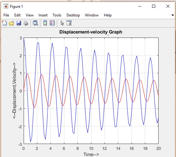
plot(t,results(:,1),'r')
hold on
plot(t,results(:,2),'b')
xlabel('Time-->')
ylabel('<--Displacement,Velocity-->')
title('Displacement-velocity_.Graph')
grid on  

ct = 1;
figure(2)
for i = 1:length(results(:,1))
    x0 = 0;
    y0 = 0;
    x1 = L*sin(results(i,1));
    y1 = -L*cos(results(i,1)); 
    plot([-1.5 1.5],[0 0],'linewidth',2,'Color','g')
    hold on
    plot([x0 x1],[y0 y1],'LineWidth',1,'Color','b')
    plot(x1,y1,'o','MarkerSize',30,'Color','r') 
    axis([-2 2 -2 2]) 
    xlabel('<--Motion_.Of_.Pendulum-->')
    ylabel('Plot')
    title('The_.Motion_.Of_.A_.Simple_.Pendulum_.With_.Damping')
    grid on
    M(ct) = getframe(gcf);
    hold off
    ct = ct+1;
end

movie(M);
videofile = VideoWriter('Harmonic Motion Of simple Pendulum.avi');
open(videofile)
writeVideo(videofile,M)
close(videofile)
 

    

• EXPLANATION OF CODE :

1. clear all : To clear all values in the workspace
2. close all : close all figures
3. clc : To clear all writings in the command window
4. b = .05 : Damping coefficient
5. g = 9.81 : Gravity
6. m = 1 : Mass of the pendulum
7. L = 1 : Lenght of the pendulum
9. t_span = linspace(0,20,100) : Its the time span between 0-20 seconds where there are 100 values with equal intervals .
11. theta_0 = [0;3] : Initial condition where angular displacement is '0' and angular velocity is '3' .
12. [t,results] = ode45(@(t,theta) ode_func(t,theta,b,g,m,L),t_span,theta_0) : ode45 is used to integrate the given function with the integration limit of t_span (0-20) and given initial values of angular displacement and angular velocity . Command used to find the output of 't' which is time and 'results' are the values of theta1 and theta2 . The values which are needed to find are being put after the ode45 command .
14. figure(1) : Comand used to create a figure named figure 1 .
15. plot(t,results(:,1),'r') : Command used to plot the graph between 't' and results in 1st column with color red .
16. hold on : Command used to hold the plots in one figure without being overwritten .
17. plot(t,results(:,2),'b') : Command used to plot the graph between 't' and results in 2nd column with color red .
18. xlabel('Time-->') : Command used to label x-axis as 'Time-->'
19. ylabel('<--Displacement,Velocity-->') : Command used to label y-axis as '<--Displacement,Velocity-->'
20. title('Displacement-velocity_.Graph') :
21. grid on : It activate the grid on the graph .
23. ct = 1 : Command used to create Frame number 1 .
24. figure(2) : Command used to create figure 2 .
25. for i = 1:length(results(:,1)) : Its a command used to start the loop with the lenght of '1' to 'results(:,1)' .
26. x0 = 0
    y0 = 0
    x1 = L*sin(results(i,1))
    y1 = -L*cos(results(i,1)) : These are the co-ordinates to create the pendulum; 'x1' and 'y1' are found by trignometry .
27. plot([-1.5 1.5],[0 0],'linewidth',2,'Color','g') : Command used to plot a line with linewidth of 2 mm and color of green with co-ordinates (-1.5,0)and(-1.5,0) .
28. hold on :
29. plot([x0 x1],[y0 y1],'LineWidth',1,'Color','b') : Command used to plot a line with linewidth of 1 mm and color of blue with co-ordinates (x0,y0)and(x1,y1) .
30. plot(x1,y1,'o','MarkerSize',30,'Color','r') : Command used to mark a point as 'o' with the marksize of 30mm and color of red with co-ordinates (x1,y1) .
31. axis([-2 2 -2 2]) : Command used to set the axis of graph with limits; x-axis (-2,2) and y-axis(-2,2) .
32. xlabel('<--Motion_.Of_.Pendulum-->') : Command used to label x-axis as '<--Motion_.Of_.Pendulum-->'
33. ylabel('Plot') : Command used to label y-axis as 'plot'
34. title('The_.Motion_.Of_.A_.Simple_.Pendulum_.With_.Damping') : Command used to title the graph as 'The motion of a simple pendulum with damping'
35. grid on :
36. M(ct) = getframe(gcf) : Command used to get seperate frames for each round of loops and saved in M(ct) .
37. hold off : To de-activate the hold on command till now so that next loop will be done in next frame .
38. ct = ct+1 : Command used to create succeeding frames; in each frames each loop is saved .
39. end : Commad used to close the loop .
41. movie(M) : Command used to create a movie with all the frames from the loop ,saved in 'M'
42. videofile = VideoWriter('Simple Pendulum with Damping'.avi') : Command used to create video ,in which the 'video name-Simple Pendulum with Damping' and 'video format -avi' is edited in paranthesis ,it can also be made into uncompressed video by editing the videowriter as -'Simple Pendulum with Damping.avi','uncompressed avi'- where the video will have the size of 64 plus mega bytes ,since i got it in 1.30 mega bytes without much quality difference in the animation video
44. open(videofile) : Opens the videofile .
45. writeVideo(videofile,M) : Command used to write all the codeing done into the videofile .
46. close(videofile) : Command used to close the videofile .

2. Outputs

• 
• Youtube : https://youtu.be/ZIlosUZUBQA
• Google drive : https://drive.google.com/file/d/18_BZPtVlY4goNkYLF16nyL0cYt50j-hv/view?usp=sharing

3. ERRORS FACED WHILE PROGRAMMING

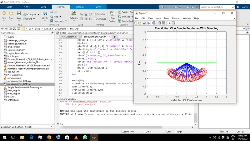
• Forgot to add hold off : I forgot to add hold off command and got below plot .so after adding hold off i got the result .

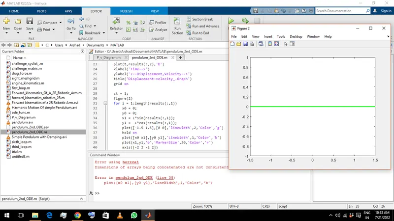
• x1 = L*sin(results(:,1))

y1 = -L*cos(results(:,1)) : I used ':', instead of using 'i'; in the equation in the loop . when corrected i got the desired result .