Week 3 - Solving second order ODEs
introduction: program in MATLAB to compute the ordinary differential equations of motion of a simple pendulum with damping.
1.main code:
% coding to compute the simple pendulum differential equations & simulate the motion of simple pendulum.
clear all
close all
clc
% defining input variables

b= 0.05; % damping coefficient(Nm/s)
g= 9.81; % accelaration due to gravity (m/s^2)
l= 1; % length of the pendulum string(m)
m= 1; % mass of the Bob(kg)
% initial condition angular displacement & angular velocity of pendulum bob

theta_0= [0;5];
% time points
t_span= linspace(0,10,400);
% solve ODE
[t,results]= ode45(@(t,theta)ode_function(t,theta,b,g,l,m),t_span,theta_0);

% plotting
figure(1)
hold on
plot(t,results(:,1),'color','g','linewidth',3)
plot(t,results(:,2),'color','b','linewidth',2)
xlabel('time in seconds')
ylabel('plot')
title('damped harmonic motion of pendulum')
legend('angular displacement','angular velocity')

angle = results(:,1);

% coordinates (defining known fixed joint positions)

x0 = 0;
y0 = 0;
plot(x0,y0,'Marker','o')
% determining the position of pendulum bob in the space using for loop command/instructions
ct=1;
for i = 1:length(angle)
    figure(2)

    THETA= angle(i);

    x = l*sin(THETA);
    y = -l*cos(THETA);

    % plotting

    plot([x0 x],[y0 y],'linewidth',3)
    hold on
    plot(x,y,'marker','o','MarkerSize',30,'MarkerFaceColor','g')
    hold off
    axis([-2 2 -2 2])
    M(ct)=getframe(gcf);
    ct=ct+1;
end
movie(M)
videofile=VideoWriter('forward_kinematics_simple_pendulum.avi','uncompressed avi');
open(videofile)
writeVideo(videofile,M)
close(videofile)
2.function script:
% function template correspond to mathematical expression in main piece ofcode
function[dtheta_dt] = ode_function(t,theta,b,g,l,m)
theta1=theta(1);
theta2=theta(2);
dtheta1_dt=theta2;
dtheta2_dt=-(b/m)*theta2-(g/l)*sin(theta1);
dtheta_dt=[dtheta1_dt;dtheta2_dt];
end
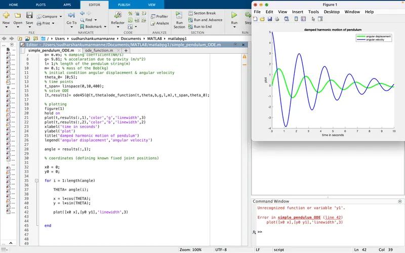
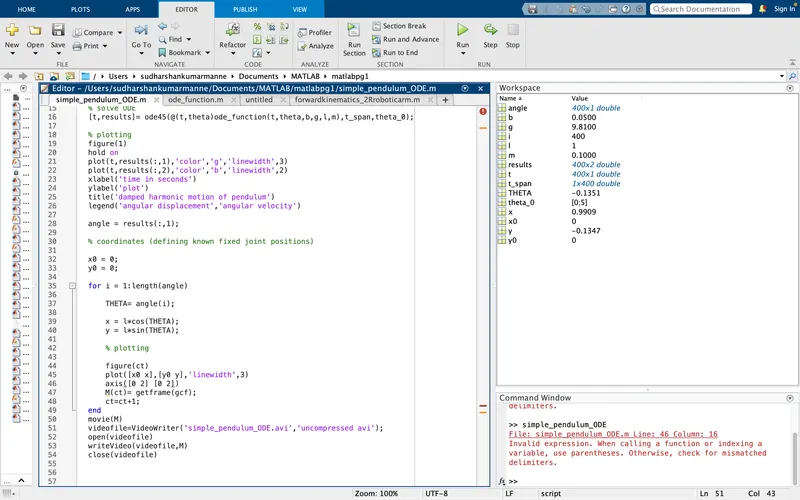
screen shots of Errors in coding:
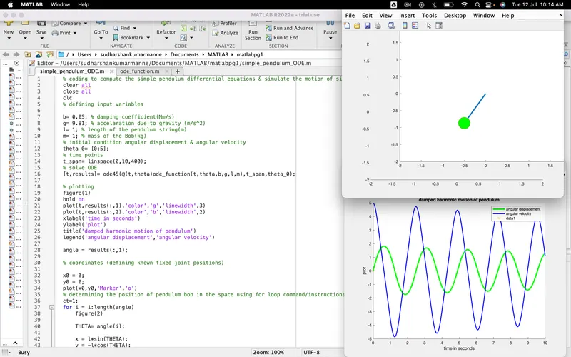
screen shots of output graph & simulation of simple pendulum ODE:
explanation:
- firstly, defined input geometric parameters & standard emperical constants for simple pendulum, such as length of the string(l), mass of the bob(m) & damping coefficient(b) , acceleration due to gratvity(g).
- in addition, assigned the initial condition of angular displement & angulur velocity of the pendulum bob in space such as 0 & 5 respectively interms of an array as theta_0.
- as well as defined/assigned desired time span & time points for sumulation of pendulum as 10 sec & 400 values interms of an array using linspace command.
- furtherly used a standard inbuilt function command such as ODE45 to solve the ordinary differential equations of motion inorder to obtain output varibles such as angular displacement & velocity w.r.t interms of array [t,results].
- such that using plot command plotted a graph for the variation of output angular displacement & velocity w.r.t time as shows the behaviour of motion exhibited by the simple pendulum.
- moreover defined/assigned initial positions of pendulum bob as x0=0,y0=0 & in order to determine the further positons achieved/reached by the pendulum bob in space , such that used kinematic equations follows the defined for loop instructions w.r.t THETA values obtained from ODE45 results.
- generated a geometrical figure for sumulation using a plot command as well as marker command with specific size for simple pendulum string & bob w.r.t to coordinate positiones on axes(X&Y) in a range of [-2 2].
- Eventually created an animation/simulation of simple pendulum motion with damping effect , using the commands getframe(gcf),counter variable(ct) & as well as the video writing commands format such as movie(M),videoWriter& writeVideo respectively.
Errors:
- faced errors while programming & their execution such as unrecognised/ unassigned variable (y1) is used instead of assigned variable (y) in the plotting command line for pendulum string positioning. so that rectified by replacing as 'y' variable.
- in addition , error made in axis command line while representing the ranges of axes (x&y) in plotting, such as used two seperate arrays ([-2 2] [-2 2]) instead of using a common array ([ -2 2 -2 2]), such that rectified accordingly.
inference:
- hence obtained an animated vedio of simulation of simple pendulum motion, using the MATLAB programming.
- as per the output results of graph & simulation, observed that the behaviour of motion of simple pendulum is harmonic in nature & the output funtions such as angular displacement & velocities w.r.t time are sinusoidal in nature.
- moreover as per the analysis of output behaviour of motion, there would be a minor daming effect on motion of the simple pendulum.
output animation video :
https://drive.google.com/file/d/1Hoah8h_pVIb8AUMNACUt8PpwoLiJ9BtE/view?usp=sharing