Week 3 - Solving second order ODEs

AIM:

• To solve the ordinary differential equation(ODE) of second order of simple pendulum in MATLAB.
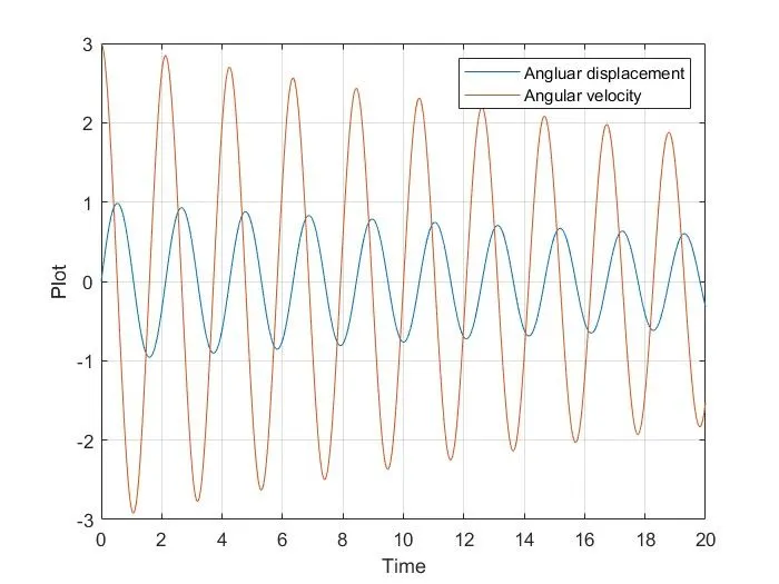
• To create a plot for variation of angle(theta) and angular velocity.
• To calculate position of simple pendulum varying with time(t) and angle(theta).
• To simulate an animation using the positions of simple pendulum.

General Procedure:

• Create a script file in MATLAB program.
• Use basic commands to clear,close all variables and clear command window.
• Save the Script file in correct directory path as same as function file should be saved in same directory path.

EXPLANATION:

• A simple pendulum is oscillated and inital conditions are noted down.
• Pendulum gradually oscillates down varying with time and rests.
• Final time taken for oscillation is noted.
• From given condition and ODE,all results like angle(theta), angular velocity & angular acceleration can be calculated varying with time.

CODING EXPLANATION:

• Initial conditons like initial angluar displacement,time taken i.e., total time taken for oscillation,damping coefficient,mass of the pendulum,gravity,angular velocity is given.
• Here,ODE is given as second order differential equation.
• MATLAB has in-built odesolvers like ode23,ode45 etc based on Runge-Kutta method.
• Using one of the MATLAB in-built command ode45,this ODE can be solved.
• ode45 can solve medium order equation
• Second order equation is converted to first order equation and conditions are applied.
  • theta1=theta(1)

    theta2=theta(2)

    dtheta1_dt=theta2

    dtheta2_dt=-(b/m)*theta2 - (g/l)*sin(theta1);

    dtheta_dt=[dtheta1_dt; dtheta2_dt];
• From solved equation,angle(theta) and angular velocity varying with time is obtained.
  • ode45 command described as[t,y]=ode45(odefunc,t_span,y0)
  • [t,results]=ode45(@(t,theta) ode_func(t,theta,b,g,l,m),t_span,theta_0)
• From these,a graph is plotted for angular veloctiy and angular displacement function as time.

Animation:

• Initial condition of pendulum is given such as length of the string,angular displacement.
• Final position of pendulum can be calculated from
  • x1=l*sin(results(i,l))
  • y1=l*cos(results(i,1))
• Graph is plotted for each and every postion of pendulum.
• Using pause and getframe command,all plotted graphs are in motion and stored in a M.
• Using videoWriter command videofile name & format is given.
• Open videofile,Write the captured images in the videofile & close the file.

CODING:

close all
clear all
clc

%solving higher order differential equation
b=0.05;
g=9.81;
l=1.0;
m=1;

%Initial condition
theta_0=[0;3];

%time points
t_span=linspace(0,20,500);

%solve ode
[t,results]=ode45(@(t,theta) ode_func(t,theta,b,g,l,m),t_span,theta_0);
figure(1)
plot(t,results(:,1))
hold on
plot(t,results(:,2))
grid on
xlabel('Time')
ylabel('Plot')
legend('Angluar displacement','Angular velocity')



%Animation
x=0;
y=0;
ct=1;
for i=1:length(t_span);

x1=l*sin(results(i,l));
y1=l*cos(results(i,1));
figure(2)

plot([-x1 x],[-y1 y],'-o')
axis([-1.2 1 -2 0.5])
grid on
pause(0.1)
M(ct)=getframe(gcf);
ct=ct+1;
end

movie(M)
videofile = VideoWriter('Pendulum.avi','Motion JPEG AVI')
open(videofile)
writeVideo(videofile,M)
close(videofile)

Function file:

function[dtheta_dt]= ode_func(t,theta,b,g,l,m)

theta1=theta(1)
theta2=theta(2)
dtheta1_dt=theta2
dtheta2_dt=-(b/m)*theta2 - (g/l)*sin(theta1);
dtheta_dt=[dtheta1_dt; dtheta2_dt];
end

RESULT:

• Graph for angular displacement and angular velocity with time is plotted.
• Simulation of pendulum is created.

https://youtu.be/zLHMJglP_OE