Project 2 - Rankine cycle Simulator
AIM:
- To write a code to find all the points in the Rankine cycle from XSteam file in MATLAB program.
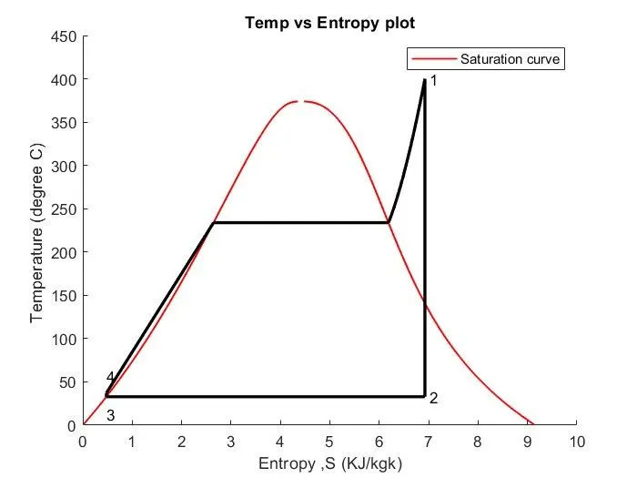
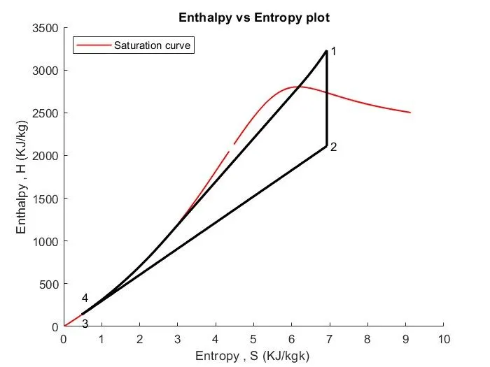
- To plot T-s and h-s diagram and saturation curve line in the graph.
General Procedure:
- Open a script file in the MATLAB command.
- Save the file in the same directory as function file.
- Use basic commands to clear,close all the variables and clear the command window.
EXPLANATION:
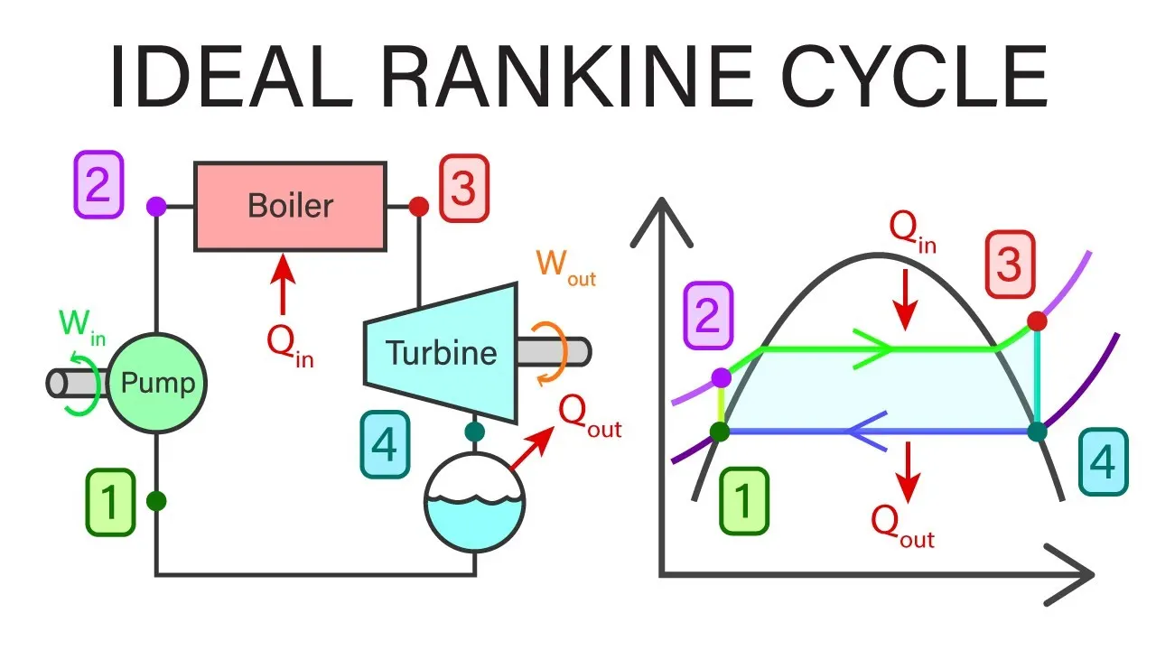
The Rankine cycle or Rankine Vapor Cycle is the process widely used by power plants such as coal fired power plants or nuclear reactors. In this mechanism, a fuel is used to produce heat within a boiler, converting water into steam which then expands through a turbine producing useful work.This thermodynamic cycle is used to convert heat energy to mechanical energy which is used to produce electricity using electric generators.
Pump:
Compression of the fluid into high pressure using pump.It takes work.Here Work is given to pump to compress the fluid.
W P = h4 – h3
B
BOILER:
The compressed fluid is heated to the final temperature (which is at boiling point), therefore, a phase change occurs—from liquid to vapor.
Qadd = h1 – h4
Turbine:
Expansion of the vapor in the turbine.
WT = h1 – h2
Condenser:
Condensation of the vapor in the condenser (where the waste heat goes to the final heat sink (the atmosphere or a large body of water.
Q rej = h2 – h3
- 1-2-3 Isobaric Heat Transfer. High pressure liquid enters the boiler from the feed pump (1) and is heated to the saturation temperature (2). Further addition of energy causes evaporation of the liquid until it is fully converted to saturated steam (3).
- 3-4 Isentropic Expansion. The vapor is expanded in the turbine, thus producing work which may be converted to electricity. In practice, the expansion is limited by the temperature of the cooling medium and by the erosion of the turbine blades by liquid entrainment in the vapor stream as the process moves further into the two-phase region. Exit vapor qualities should be greater than 90%.
- 4-5 Isobaric Heat Rejection. The vapor-liquid mixture leaving the turbine (4) is condensed at low pressure, usually in a surface condenser using cooling water. In well designed and maintained condensers, the pressure of the vapor is well below atmospheric pressure, approaching the saturation pressure of the operating fluid at the cooling water temperature.
- 5-1 Isentropic Compression. The pressure of the condensate is raised in the feed pump. Because of the low specific volume of liquids, the pump work is relatively small and often neglected in thermodynamic calculations.
The thermodynamic efficiency of this cycle can be calculated by the following formula:
CODE EXPLANATION:
- Use the function file to extract points for rankine cycle.
- Extract points such as Enthalpy,Entropy,Pressure and Temperature from the function file.
- Heat Rejection and Heat addition is calculated.
- Work of turbine and Work of Pump is calculated.
- Thermal Efficiency of Rankine cycle is calculated.
- Specific Steam Consumption is calculated.
CODING:
clear all
close all
clc
%Rankine cycle
fprintf('\n RANKINE CYCLE SIMULATOR')
fprintf('\n 1-2 Isentropic expansion in Turbine')
fprintf('\n 2-3 Constant Pressure Heat Rejection in the condenser')
fprintf('\n 3-4 Isentropic Compression in the Pump')
fprintf('\n 4-1 Constant Pressure Heat addition in the Boiler')
%Given inputs for rankine cycle

%Turbine inlet temperature @ degree C
T1=input('\n Enter the tempertaure inlet Turbine (in C)')

%Turbine Inlet pressure @ bars
P1=input('Enter the Turbine inlet Pressure (in bars)')

%Turbine Outlet Pressure @ bars
P2=input('Enter the Condenser inlet Pressure (in bars)')

%At state point 1
H1=XSteam('h_pT',P1,T1);

S1=XSteam('s_pT',P1,T1);

%At state point 2
S2=S1;

sf2=XSteam('sL_p',P2);
sg2=XSteam('sV_p',P2);
x2=(S2-sf2)/(sg2-sf2);
hf2=XSteam('hL_p',P2);
hg2=XSteam('hV_p',P2);
H2=hf2+(x2*(hg2-hf2));

% State 3
P3 = P2;
S3= XSteam('sL_p', P3);
H3 = XSteam('hL_p', P3);

% State 4
S4 = S3;
P4 = P1;

% Work done by turbine
Wt = H1 - H2;

% Work done to run pump
v3 = XSteam('vL_p', P3);
Wp = v3*(P4 - P3)*100;
H4 = H3 + Wp;

%net work
Wnet = Wt - Wp;

%Heat into the system
Qin = H1 - H4;

%Heat out of the system
Qout = H2 - H3;

%Thermal efficiency
eff = (Wnet/Qin)*100;

%Specific Steam Consumption
%SSC = mass flow rate/power
SSC = (3600/Wnet);


%Calculating temperatures at the state points
T3 = XSteam('Tsat_p', P3);
T2 = T3;
Cp4 = XSteam('Cp_ps', P4, S4);
Cv4 = XSteam('Cv_ps', P4, S4);
k = Cp4/Cv4;
T4 = T3/((P3/P4)^((k-1)/k));

%Calculating temperature, entropy and enthalpy at the vapour and liquid
%line for plotting
T6 = XSteam('Tsat_p', P1);
S5 = XSteam('sL_p', P1);
S6 = XSteam('sV_p', P1);
H5 = XSteam('hL_p', P1);
H6 = XSteam('hV_p', P1);
T5 = T6;

%Plotting the saturation curve
T = linspace(1,375,1000);
for i = 1:length(T)

sf(i) = XSteam('sL_T', T(i));
sg(i) = XSteam('sV_T', T(i));
hf(i) = XSteam('hL_T', T(i));
hg(i) = XSteam('hV_T', T(i));
end

%Plotting T-s diagram
figure(1)
hold on
plot(sf, T, 'r','linewidth',1)
plot(sg, T, 'r','linewidth',1)
plot([S1 S2], [T1 T2], 'k', 'linewidth', 2)
plot([S2 S3], [T2 T3] ,'k', 'linewidth', 2)
plot([S3 S4], [T3 T4], 'k', 'linewidth', 2)
plot([S4 S5], [T4 T5], 'k', 'linewidth', 2)
plot([S5 S6], [T5 T6], 'k', 'linewidth', 2)
sc1 = linspace(S6, S1, 1000);
for l = 1:length(sc1)
 Tc1(l) = XSteam('T_ps', P1, sc1(l));
end
plot(sc1, Tc1, 'k', 'linewidth', 2)
text(S1+0.1, T1, '1')
text(S2+0.1, T2, '2')
text(S3, T3-20, '3')
text(S4, T4+20, '4')
title('Temp vs Entropy plot')
xlabel('Entropy ,S (KJ/kgk)')
ylabel('Temperature (degree C) ')
legend('Saturation curve')


%Plotting h-s diagram
figure(2)
hold on
plot(sf, hf, 'r', 'linewidth', 1)
plot(sg, hg, 'r',  'linewidth', 1)
plot([S1 S2], [H1 H2], 'k', 'linewidth', 2)
plot([S2 S3], [H2 H3], 'k', 'linewidth', 2)
plot([S3 S4], [H3 H4], 'k', 'linewidth', 2)
hc = linspace(H4, H5, 100);
for k = 1:length(hc)
sch(k) = XSteam('s_ph', P1, hc(k));
end
plot(sch,hc, 'k', 'linewidth', 2)
plot([S5 S6], [H5 H6], 'k', 'linewidth', 2)
for m = 1:length(sc1)
hc1(m) = XSteam('h_ps', P1, sc1(m));
end
plot(sc1, hc1, 'k', 'linewidth', 2)
text(S1+0.1, H1, '1')
text(S2+0.1, H2, '2')
text(S3, H3-100, '3')
text(S4, H4 +200, '4')
title('Enthalpy vs Entropy plot')
xlabel('Entropy , S (KJ/kgk) ')
ylabel('Enthalpy , H (KJ/kg)')
legend('Saturation curve','location','northwest')


% Displaying Results
disp(' RESULTS');
fprintf('At State Point 1:\n');
fprintf('p1: %8.3f bar\n', P1);
fprintf('T1: %8.3f C\n', T1);
fprintf('h1: %8.3f KJ/kg\n', H1);
fprintf('s1: %8.3f KJ/kgK\n\n', S1);
fprintf('At State Point 2:\n');
fprintf('p2: %8.3f bar\n', P2);
fprintf('T2: %8.3f C\n', T2);
fprintf('h2: %8.3f kJ/kg\n', H2);
fprintf('s2: %8.3f kJ/kgK\n', S2);
fprintf('x2: %8.3f\n\n', x2);
fprintf('At State Point 3:\n');
fprintf('p3: %8.3f bar\n', P3);
fprintf('T3: %8.3f K\n', T3);
fprintf('h3: %8.3f kJ/kg\n', H3);
fprintf('s3: %8.3f kJ/kgK\n\n', S3);
fprintf('At State Point 4:\n');
fprintf('p4: %8.3f bar\n', P4);
fprintf('T4: %8.3f K\n', T4);
fprintf('h4: %8.3f KJ/kg\n', H4);
fprintf('s4: %8.3f kJ/kgK\n\n', S4);
fprintf('Turbine Work: %8.3f kJ/kg\n', Wt);
fprintf('Pump Work: %8.3f kJ/kg\n', Wp);
fprintf('Wnet: %8.3f kJ/kg\n', Wnet);
fprintf('Efficiency: %8.3f Percent \n ', eff);
fprintf('S.S.C: %8.3f kJ/kWh', SSC);
OUTPUT:
 RANKINE CYCLE SIMULATOR
 1-2 Isentropic expansion in Turbine
 2-3 Constant Pressure Heat Rejection in the condenser
 3-4 Isentropic Compression in the Pump
 4-1 Constant Pressure Heat addition in the Boiler
 Enter the tempertaure inlet Turbine (in C)400

T1 =

   400

Enter the Turbine inlet Pressure (in bars)30

P1 =

    30

Enter the Condenser inlet Pressure (in bars)0.05

P2 =

    0.0500

 RESULTS
At State Point 1:
p1:   30.000 bar
T1:  400.000 C
h1: 3231.571 KJ/kg
s1:    6.923 KJ/kgK

At State Point 2:
p2:    0.050 bar
T2:   32.875 C
h2: 2110.708 kJ/kg
s2:    6.923 kJ/kgK
x2:    0.814

At State Point 3:
p3:    0.050 bar
T3:   32.875 K
h3:  137.765 kJ/kg
s3:    0.476 kJ/kgK

At State Point 4:
p4:   30.000 bar
T4:   36.935 K
h4:  140.776 KJ/kg
s4:    0.476 kJ/kgK

Turbine Work: 1120.863 kJ/kg
Pump Work:    3.011 kJ/kg
Wnet: 1117.852 kJ/kg
Efficiency:   36.167 Percent
 S.S.C:    3.220 kJ/kWh>>
RESULT:
- Enthalpy,Entropy,Temperature and Pressure of all the points are calculated using function file.
- All the points are plotted in the graph.