Week 3 - Solving second order ODEs

Aim: Transient behaviour of simple pendulum

Theory: A point mass attached to a light inextensible string and suspended to a fixed support is called a simple pendulum. A verticle line passing through the fixed support is the mean position of the simple pendulum.

A vertical distance between pount of suspension and center of mass of a suspended body is called length of the simple pendulum.

Governing equation:

`(d^2theta)/dt^2+b/m(d theta) /dt + g/lsintheta`

where,

l = length of the pendulum

m = mass of the bob

b = damping coefficient

g = gravity

Breaking down the above second order differential equation to first order differential equation

`theta = theta1`

`(d theta)/dt = (d theta1)/dt = theta2`

`(d^2theta)/dt^2 = (d^2theta1)/dt^2 = (d^2theta2)/dt`

`(d theta2)/dt = -b/mtheta2 - g/lsintheta`

#Code

clear all
close all
clc
% Declaration of the varible
l=1;     % length of the string
m=1;     % mass of the bob
b=0.05;  % Damping coefficient
g=9.8;   %acceleration due to gravity
ct=1;
%initial Condition
theta_0 = [0,3];
%time points
t_span = linspace(0,20,200);
%solving ode
%calling the the pendulum_func using ode45 function
[t,result] = ode45(@(t,theta) pendulum_fun(t,theta,b,g,l,m),t_span,theta_0);
plot(t, result(:,1))
hold on
plot(t, result(:,2))
xlabel('time')
ylabel('amplitude')
legend('Angular Displacement','Angular Velocity')
grid on;
theta2=result(:,1);
% creating animation
for i =1:length(theta2);
    theta_x=theta2(i);
    %initial position of the pendulum
    x0=0;
    y0=0;
    %pendulum position in different angle
    x1= l*sin(theta_x);
    y1= -l*cos(theta_x);
    % ploting the simple pendulum
     figure(2)
     %ploting the supporting rod 
     plot([-0.5 0.5],[0 0],'color','b','linewidth',3);
     hold on;
     %ploting the length of the pendulum
     plot([x0 x1],[y0 y1],'color','r','linewidth',2);
     hold on;
     % ploting the bob of the pendulum
     plot(x1,y1,'o','markers',15,'markerfacecolor','y')
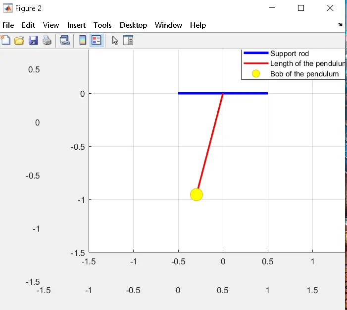
     title('Animation of Simple Pendulum');
     legend('Support rod','Length of the pendulum','Bob of the pendulum');
     hold off;
     grid on;
     %providing axis for the animation
     axis([-1.5 1.5 -1.5 0.5]);
     pause(0.002)
    M(ct)= getframe(gcf);
    %countering the loop
    ct= ct+1;  
end
%inserting frames in the animation to make movie
movie(M)
%creating the .avi file
videofile = VideoWriter('Simple_pendulum.avi','uncompressed avi');
open(videofile);
writeVideo(videofile,M);
close(videofile);

#pendulum_fucn code

function[dtheta_dt]=pendulum_fun(t,theta,b,g,l,m)
theta1 = theta(1);
theta2=theta(2);
dtheta1_dt= theta2;
dtheta2_dt = -(b/m)*theta2-(g/l)*sin(theta1);
dtheta_dt = [dtheta1_dt; dtheta2_dt];
end

#Animation

#Graph

Time vs Amplitude

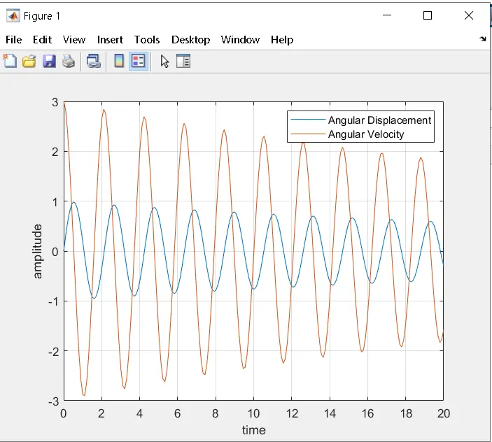
Pendulum motion