Week 3 - Solving second order ODEs

AIM

Solving a second order ordinary differential equation of simple pendulum and showing the effect of damping by an animation.

OBJECTIVE

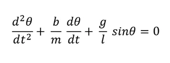
• To convert second order ordinary differential equation to 1^st order ordinary differential equation.
• To create the function using MATLAB in-built function for solving ordinary differential equation.
• To plot the displacement and velocity damping through the time stipulated time of simulation.
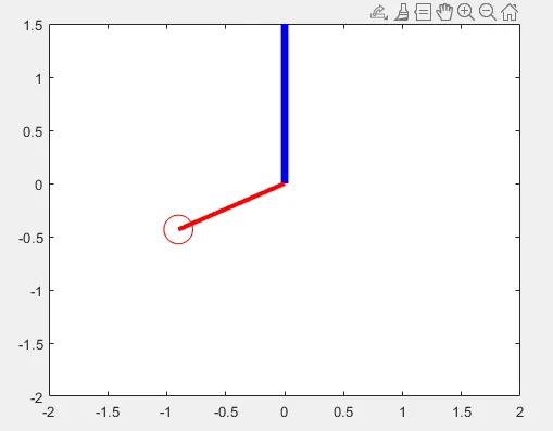
• To make the animation simple pendulum.

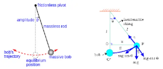
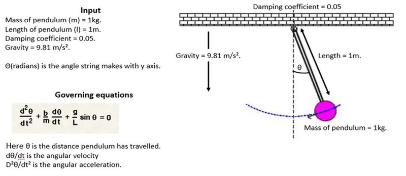
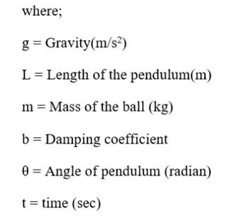
Description & governing equation.

We saw in the chapter introduction that second-order linear differential equations are used to model many situations in physics and engineering. In this section, we look at how this works for systems of an object with mass attached to a vertical spring and an electric circuit containing a resistor, an inductor, and a capacitor connected in series. Models such as these can be used to approximate other more complicated situations; for example, bonds between atoms or molecules are often mode led as springs that vibrate, as described by these same differential equations.

Simple Harmonic Motion

Consider a mass suspended from a spring attached to a rigid support. (This is commonly called a spring-mass system.) Gravity is pulling the mass downward and the restoring force of the spring is pulling the mass upward. these two forces are equal, the mass is said to be at the equilibrium position. If the mass is displaced from equilibrium, it oscillates up and down. This behavior can be mode led by a second-order constant-coefficient differential equation.

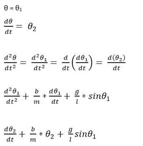
CODE EXPLANATION :

1. The code starts with the inputs which are provided in the problem. Then we make time domain for which the whole code is going to run. It was done by ‘linspace’ command 0 to 17 seconds with 100 value in between.
2. After that we provide the initial condition for the angular displacement and velocity which is column vector form, because we need to calculation the both value from the equation of motion for plotting purpose.
3. The code comprises of function which solves the second order differential equation which is taken inside the main code. The main code has another function which calculates is used ,in the first plot first the array of data for time and displacement.
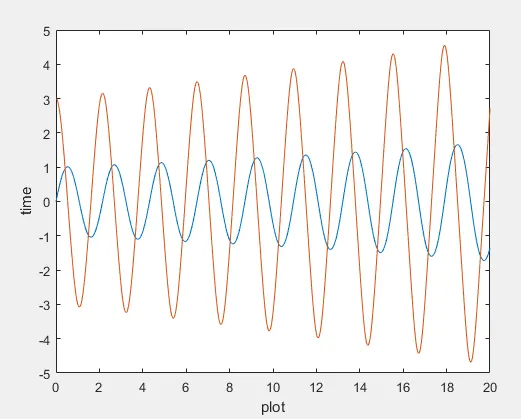
4. After calculation plotting is done in which subplot command is used ,in the first plot first column is plotted and in second subplot second column is plotted with respect to time.
5. Then we are changing the polar co-ordinate to cartesian co-ordinate because we have used ‘sind’ command in function.
6. Then we have created a for loop for which we are creating the frame motion for the simple pendulum and saved in the movie.

The code is given as:

%input
b = 0.05;
g = 9.81;
l = 1;
m = 1;

% interial conditon
theta_0 = [0;3];

%time points
t_span = linspace(0,20,500);

%SOLVE ODE
[t,results]= ode45(@(t,theta) ode_func(t,theta,b,g,l,m),t_span,theta_0);

plot(t,results(:,1))
hold on
plot(t,results(:,2))
xlabel('plot')
ylabel('time')

figure(2)
theta = results(:,1);
ct=1;
for i=1:length(theta)

    x0 = 0;
    y0 = 0;

    x1 = -1*sin(theta(i));
    y1 = -1*cos(theta(i));

    plot([0 0],[1.5 0],'linewidth',5,'color','b')
    hold on
    plot([x0 x1],[y0 y1],'LineWidth',3,'Color','r')
    axis([-2 2 -2 1.5])
    plot(x1,y1,'o','MarkerSize',20,'Color','r')
    pause(0.1)
    M(ct)= getframe(gcf);
    hold off
    ct=ct+1;
end
%making the video file
movie(M)
videofile=VideoWriter('simple_pendulum.avi')
open(videofile)
writeVideo(videofile,M)
close(videofile)

CODE FOR FUNCTION USED IN PROGRAM:

function [dtheta_dt] = ode_func(t,theta,b,g,l,m)

theta1 = theta(1);
theta2 = theta(2);
dtheta1_dt = theta2;
dtheta2_dt = (b/m)*theta2-(g/l)*sin(theta1);
dtheta_dt = [dtheta1_dt; dtheta2_dt];
end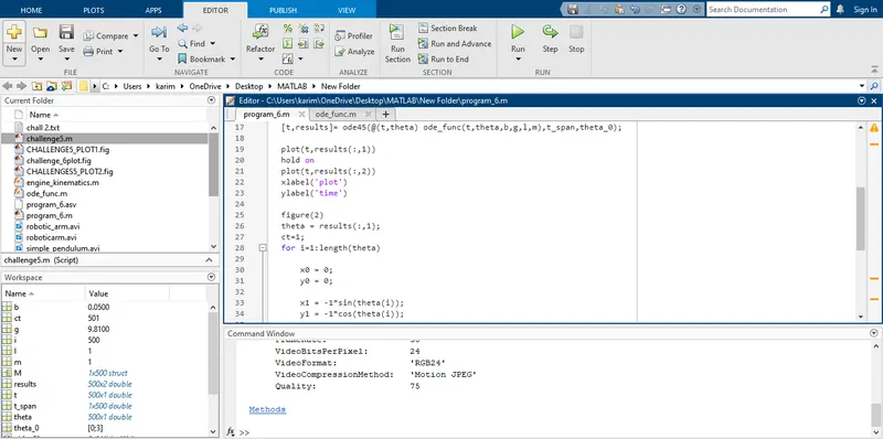

OUTPUT GRAPE:

RESULT:

https://youtu.be/D0b9JbSDNIA

CONCLUSION:

• The graph of angular displacement and angular velocity plotted for the pendulum is sinusoidal in nature. the amplitude of motion reduces gredually as the motion is damped.