Week 3 - Solving second order ODEs

TITLE: SOLVING SECOND ORDER ORDINARY DIFFERENCIAL EQUATION USING MATLAB.

OBJECTIVES:

1. To find the solution of an second order differencial equation.

2. To get the position of the pendulum as a function of time.

INTRODUCTION:

1. DIFFERENCIAL EQUATIONS:

In Mathematics, a differential equation is an equation that contains one or more functions with its derivatives. The derivatives of the function define the rate of change of a function at a point. It is mainly used in fields such as physics, engineering, biology and so on. The primary purpose of the differential equation is the study of solutions that satisfy the equations and the properties of the solutions.

2. Differential Equation Definition:

A differential equation is an equation which contains one or more terms and the derivatives of one variable (i.e., dependent variable) with respect to the other variable (i.e., independent variable).

dy/dx = f(x)

Here “x” is an independent variable and “y” is a dependent variable.

A differential equation contains derivatives which are either partial derivatives or ordinary derivatives. The derivative represents a rate of change, and the differential equation describes a relationship between the quantity that is continuously varying with respect to the change in another quantity. There are a lot of differential equations formulas to find the solution of the derivatives.

3. Ordinary Differential Equation:

An ordinary differential equation involves function and its derivatives. It contains only one independent variable and one or more of its derivatives with respect to the variable.

The order of ordinary differential equations is defined as the order of the highest derivative that occurs in the equation. The general form of n-th order ODE is given as

F(x, y, y’,…., yⁿ ) = 0

for pendulum:

where,

b = damping co-efficient.

m = mass of the body.

g = gravitational force.

L = length of a string.

4. Applications:

Differential equations have several applications in different fields such as applied mathematics, science, and engineering. Apart from the technical applications, they are also used in solving many real life problems. Let us see some differential equation applications in real-time.

1) Differential equations describe various exponential growths and decays.

2) They are also used to describe the change in return on investment over time.

3) They are used in the field of medical science for modelling cancer growth or the spread of disease in the body.

4) Movement of electricity can also be described with the help of it.

5) They help economists in finding optimum investment strategies.

6) The motion of waves or a pendulum can also be described using these equations.

The various other applications in engineering are: ­ heat conduction analysis, in physics it can be used to understand the motion of waves. The ordinary differential equation can be utilized as an application in the engineering field for finding the relationship between various parts of the bridge.

In this project we have taken an example of the motion of waves or a pendulum.

6. Simple Pendulum:

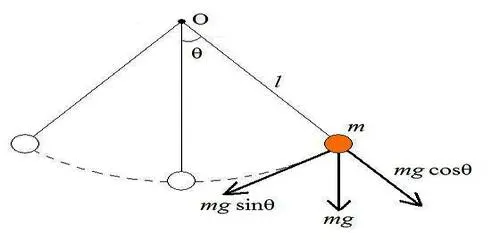
A simple pendulum can be described as a device where its point mass is attached to a light inextensible string and suspended from a fixed support. The vertical line passing through the fixed support is the mean position of a simple pendulum. The vertical distance between the point of suspension and the centre of mass of the suspended body (when it is in mean position) is called the length of the simple pendulum denoted by L. This form of the pendulum is based on the resonant system having a single resonant frequency.

7. Simple Pendulum Definition:

A simple pendulum is a mechanical arrangement that demonstrates periodic motion. The simple pendulum comprises a small bob of mass ‘m’ suspended by a thin string secured to a platform at its upper end of length L.

The simple pendulum is a mechanical system that sways or moves in an oscillatory motion. This motion occurs in a vertical plane and is mainly driven by the gravitational force. Interestingly, the bob that is suspended at the end of a thread very light somewhat we can say it is even massless. The period of a simple pendulum can be made extended by increasing the length string while taking the measurements from the point of suspension to the middle of the bob. However, it should be noted that if the mass of the bob is changed it will the period remains unchanged. Period is influenced mainly by the position of the pendulum in relation to Earth as the strength of gravitational field is not uniform everywhere.

Meanwhile, pendulums are a common system whose usage is seen in various instances. Some are used in clocks to keep track of the time while some are just used for fun in case of a child’s swing. In some cases, it is used in an unconventional manner such as a sinker on a fishing line. In any case, we will explore and learn more about the simple pendulum on this page. We will discover the conditions under which it performs simple harmonic motion as well as derive an interesting expression for its period.

8. Important Terms:

• The oscillatory motion of a simple pendulum: Oscillatory motion is defined as the to and fro motion of the pendulum in a periodic fashion and the centre point of oscillation known as equilibrium position.
• The time period of a simple pendulum: It is defined as the time taken by the pendulum to finish one full oscillation and is denoted by “T”.
• The amplitude of simple pendulum: It is defined as the distance travelled by the pendulum from the equilibrium position to one side.
• Length of a simple pendulum: It is defined as the distance between the point of suspension to the centre of the bob and is denoted by “l”.

9. About ODE45 in matlab:

ODE45 is usually the function of choice among the ODE solvers. It compares methods of orders four and five to estimate error and determine step size. ODE45 is so accurate that its default behavior is to use its interpolant to provide results at intermediate points.

10. Functions:

Both scripts and functions allow you to reuse sequences of commands by storing them in program files. Functions provide more flexibility, primarily because you can pass input values and return output values. In addition, functions avoid storing temporary variables in the base workspace and can run faster than scripts.

Function Creation:

Functions contain one or more sequential commands and can accept inputs and return outputs. To write a program with multiple lines of code, create a named function in a file.

Alternatively, if you want to define a one-line function to pass to another function—for instance, a mathematical expression to pass to the integral function—you can create an anonymous function.

Lets have a look on Program:

first thing creation of function

function [dtheta_dt] = ode_func(t,theta,b,g,l,m)

theta1 = theta(1);
theta2 = theta(2);

dtheta1_dt = theta2;
dtheta2_dt = -(b/m)*theta2 - (g/l)*sin(theta1);
dtheta_dt = [dtheta1_dt ; dtheta2_dt];

end

main code

clear all
close all
clc

%inputs
b = 0.05;
g = 9.81;
l = 1;
m = 1;

%intial condition
theta_0 = [0;3];

%time points
tspan = linspace(0,20,500);

%solving ODE
[t,result] = ode45(@(t,theta) ode_func(t,theta,b,g,l,m),tspan, theta_0);

%Plotting
figure(1)
plot(t,result(:,1))
hold on
plot(t,result(:,2))
ylabel('Plot')
xlabel('Time')
grid on

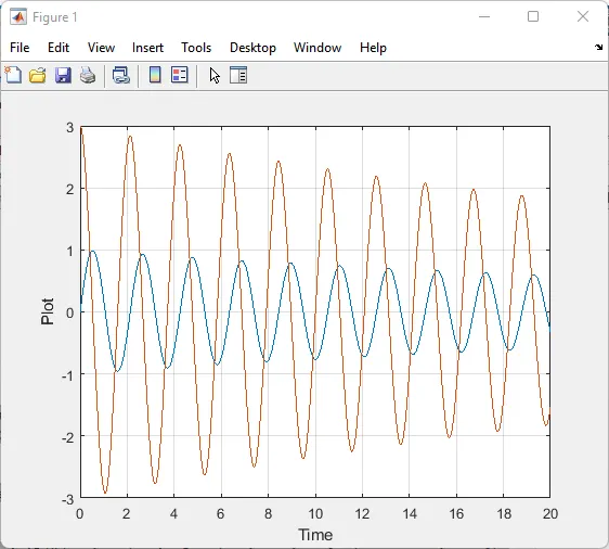
till here are able to see, above program had given some inputs, Time Span.

if we plot this function looks like,

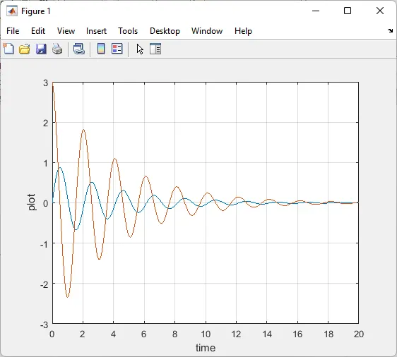
try with another values, frequency also changes.

for making an video of simple moving pendulum we need some extra program.

then the final program is look like mentioned below, with drive link of video and the program.

clear all
close all
clc

%inputs
b = 0.05;
g = 9.81;
l = 1;
m = 1;

%intial condition
theta_0 = [0;3];

%time points
tspan = linspace(0,20,500);

%solving ODE
[t,result] = ode45(@(t,theta) ode_func(t,theta,b,g,l,m),tspan, theta_0);

%Plotting
figure(1)
plot(t,result(:,1))
hold on
plot(t,result(:,2))
ylabel('Plot')
xlabel('Time')
grid on

%DEFINING VALUES FOR GIF
ct = 1;

%USING FOR LOOP
for i = 1:length(result(:,1))
    x_start = 0
    y_start = 0
    x_end = 1*sin(result(i,1))
    y_end = -1*cos(result(i,1))
    
    %plotting an GIF
    figure(2)
    plot([-1 1],[0 0],'linewidth',3)
    hold on
    plot([x_start x_end],[y_start y_end],'linewidth',3)
    hold on
    plot(x_end,y_end,'o','markersize',20,'markerfacecolor','r')
    axis([-1.5 1.5 -1.5 1.5])
    pause(0.03)
    hold off
    M(ct)=getframe(gcf)
    ct=ct+1
end

%gif of pendulum
movie(M)
videofile=VideoWriter('pendulum.avi','uncompressed AVI');

open(videofile)
writeVideo(videofile,M)
close(videofile)

video link:

https://drive.google.com/file/d/1zaKca12KtS-63x4YTlkBd_yD8zfRgwad/view?usp=sharing

https://drive.google.com/drive/folders/16JRISQr5OSzYxMQyy3_-iQ3b--UDfR8J?usp=sharing