Week 3 - Solving second order ODEs

Aim: 

Write a program in python to solve 2nd order ODE for a simple pendulum and to plot angular displacement and angular velocity graph to analyze its motion to observe transient behavior of a pendulum. 

Solution: 

Assume a simple pendulum with a pendulum bob which has a mass of m and suspended with a string.  

Now, for initial condition, θ = θ1 

Hence,

d𝜃dt =d𝜃1dt =𝜃2">dθ/dt =dθ1/dt =θ2 

Further,

d2𝜃dt2 =d2𝜃1dt 2=ddtd𝜃1dt=ddt𝜃2">d2θ/dt2 =d2θ1/dt2=d/dt(dθ1/dt)=d/dt(θ2)

2nd order ODE for mass-pendulum damping system, 

d2𝜃dt2 +bm ⋅d𝜃dt +glsin⁡𝜃1=0">d2θ/dt2 +b/m ⋅dθ/dt +g/lsin(θ1)=0

So,

d2𝜃1dt2 +bm ⋅d𝜃1dt +glsin⁡𝜃1=0">d2θ1/dt2 +b/m ⋅dθ1/dt +g/lsin(θ1)=0

d2𝜃2dt2 +bm ⋅𝜃2 +glsin⁡𝜃1=0">d2θ2/dt2 +b/m ⋅θ2 +g/lsin(θ1)=0

1st ODE, d𝜃1dt =𝜃2">dθ1/dt =θ2

2nd ODE, d𝜃2dt =−bm𝜃2−glsin⁡𝜃1">dθ2/dt =−b/mθ2−g/lsin(θ1)

Nomenclature: 

b = damping coefficient  

l = length of string, m 

m = mass of bob, kg 

g = acceleration due to gravity, m/s^2 

Θ = angular displacement   

Program: 

#Solving 2nd order ODE 
#Anvar Choksi

import numpy as np
import matplotlib.pyplot as plt 
import math
from scipy.integrate import odeint 

#function that returns d2/dt
def model(theta,t,b,g,l,m):

	theta1 = theta[0]
	theta2 = theta[1]
	dtheta1_dt = theta2
	dtheta2_dt = -(b/m)*theta2 - (g/l)*math.sin(theta1)
	dtheta_dt = [dtheta1_dt,dtheta2_dt]
	
	return dtheta_dt 

b = 0.02
g = 9.81
l = 1 
m = 0.1

#Initian Condition 
#theta_0 = [math.pi/2,0]
theta_0 = [0,3]

#time points
t = np.linspace(0,10,150)

#solve ODE
theta = odeint(model,theta_0,t,args = (b,g,l,m))

#plot results 
plt.plot(t,theta[:,0],'b-',label=r'$\frac{d\theta1}{dt} = \theta2$')
plt.plot(t,theta[:,1],'r--',label=r'$\frac{d\theta2}{dt} = -\frac{b}{m}\theta_2 - \frac{g}{l}sin\theta_1$')
plt.ylabel('plot')
plt.xlabel('time')
plt.legend()
plt.savefig('output.png')
plt.show()

# To creat animation
ct = 1
x0 = 0
y0 = 0

for i in theta[:,0]:
	x1=x0+(l*math.sin(i))
	y1=y0+(-l*math.cos(i))

	filename = str(ct)+'.png'
	ct = ct +1

	plt.figure()
	plt.plot([-1,1],[0,0],"black")
	plt.plot([x0,x1],[y0,y1],"red") 
	plt.plot(x1,y1,'o',markersize = '20')
	plt.xlim([-1.5,1.5])
	plt.ylim([-1.5,1.0]) 
	plt.savefig(filename)

Output: 

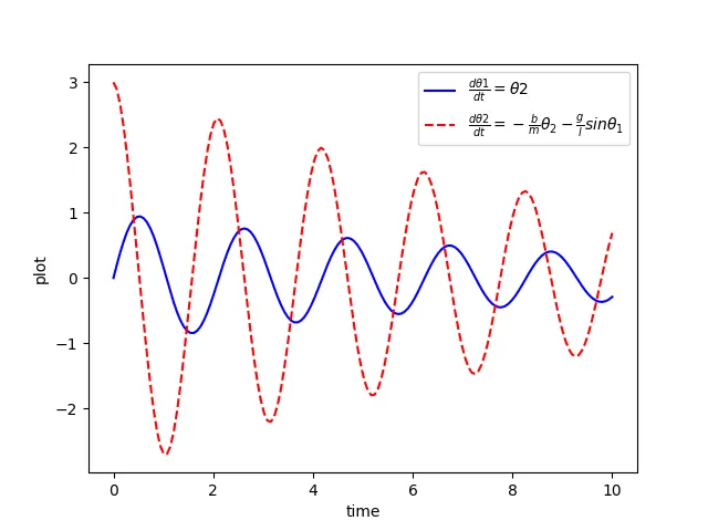
Conclusion: The effect of damping can be clearly seen from the graph as the graph of angular displacement and angular velocity displacement depicts that the motion of pendulum is gradually decreasing with time. Hence, any 2nd order ODE can be solved with python.