Week 3 - Solving second order ODEs

Aim: Solving second order Ordinary Differential Equation in Matlab

Objectives:

• To create graphical representation of Angular velocity (rad/s)/Displacement (rad) wrt time
• Creating animation file

Introduction: Second order differential equation is a specific type of differential equation that consists of a derivative of a function of order 2 and no other higher-order derivative of the function appe ars in the equation. It includes terms like y'', d²y/dx², y''(x), etc. which indicates the second order derivative of the function. Generally, we write a second order differential equation as y'' + p(x)y' + q(x)y = f(x), where p(x), q(x), and f(x) are functions of x

ODE is used to describe the transient behaviour of a system. A simple example is a pendulum the way the pendulum moves depends on the Newton’s second law. We solved this we get a second order Ordinary Differential Equation that describes the position of the "ball" w.r.t time.

Simple Pendulum

To simply define simple pendulum, it is a bob that comprises of a molecule of mass ‘m’ suspended by a massless non-expandable string of length ‘L’ in an area of space in which there is a consistent, uniform gravitationa l field, e.g. near the surface of the earth. The suspended molecule is called the pendulum bob.

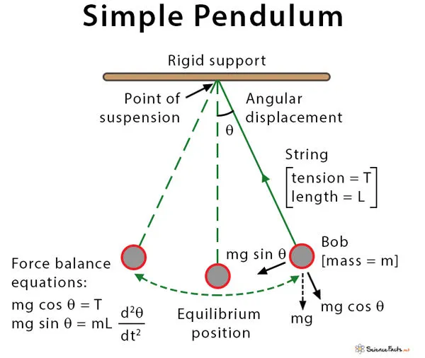
Terms

g = gravity in m/s2,

L = length of the pendulum in m,

m = mass of the ball in kg,

b=damping coefficient.

According to Newton’s second law,

F = ma (Newton’s second law)

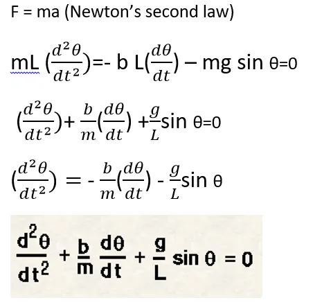
Where,

b=0.05; % damping coefficient

g=9.81; % gravity in m/s^2

l=1; % length of pendulum in m

m=0.1; % mass of ball in kg

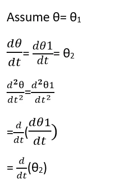
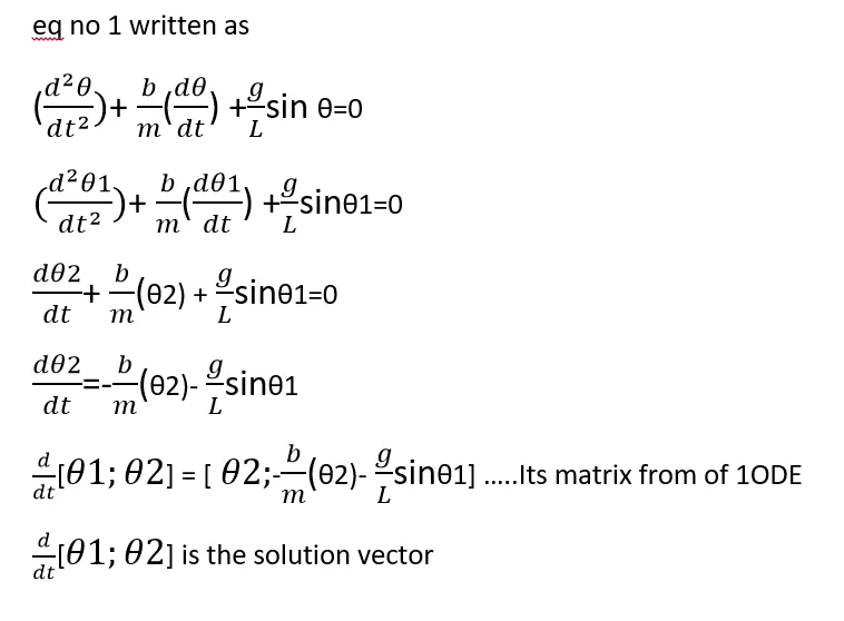
To solve in mat lab we converting this 2^nd ODE into 1^st order because the in mat lab function ode45 is solved only 1^st ODE

Program for the simple pendulam

clear all
close all
clc
%inputs 
b=0.05; % damping coefficient 
g=9.81; % gravity in m/s^2
l=1;    % length of pendulam in m
m=0.1;  % mass of ball in kg

%initial condiations
theta_0=[0;3];

%time ponits
t_span=linspace(0,20,500);

%solve ODE by using function 
[t,result]=ode45(@(t,theta) ode_func(t,theta,b,g,l,m),t_span,theta_0);


%ploting Angular velocity (rad/s)/Displacement (rad) vs time 
figure(1)
plot(t_span,result(:,1))     
hold on                    
plot(t,result(:,2))          
xlabel('time in sec')               
ylabel('Angular velocity (rad/s)/Displacement (rad)')  
legend('displacement','Angular Velocity')



%Animation of the pendulam
ct=1;                        
for i=1:length(result(:,1))  
    x0=0;                      
    y0=0;                   
    x1=1*sin(result(i,1));
    y1=-1*cos(result(i,1)); 
    figure(2)
    plot([0,0],[-1.5,0.5])   
    hold on                  
    plot([-1.5,1.5],[0,0],'LineWidth',15,'Color','black') 
    hold on 
    plot([x0 x1],[y0 y1],'LineWidth',3,'Color','r') 
    hold on
    axis ([-1.5 1.5 -1.5 0.5]) 
    plot(x0,y0,'marker','.','MarkerSize',15,'Color','g')
    plot(x1,y1,'marker','.','MarkerSize',60,'Color','g')
    M(ct)=getframe(gcf);
    
    ct=ct+1;
    hold off 
end 
% Videofile of out put
movie(M)
Videofile=VideoWriter("ode2pendulum.m",'Uncompressed AVI') 
open(Videofile) 
writeVideo(Videofile,M) 
close(Videofile)

Program for the ode Function (function_end)

function [dtheta_dt]=ode_func(t,theta,b,g,l,m)

theta1=theta(1)
theta2=theta(2)
dtheta1_dt=theta2;
dtheta2_dt=-(b/m)*theta2-(g/l)*sin(theta1);
dtheta_dt=[dtheta1_dt;dtheta2_dt];
end

Step wise explanation of Program

1.Clear Screen

• 1^st start writing the code it is important to start wirh clear all,close all,and clc
• Clear all-remove the data from workplace and freeing up system memory
• Close all-deletes the current figure or the specified fig
• Clc =clears all input and output from the command window display

2.Assigning Input Variables

as given in problem

• b=0.05; damping coefficient
• g=9.81; gravity in m/s^2
• l=1; length of pendulum in m
• m=0.1; mass of ball in kg

3.Initial conditions

To Simulate the motion between 0-20 sec, for angular displacement=0, angular velocity=3 rad/sec at time t=0.

• theta_0=[0;3];consider as angular displacement is 0 and angular velocity 3
• t_span=linspace(0,20,500);consider initial time as 0 and final time as 20 and in this time we want to study 500 position

4.ode45

ode45 is a function in MATLAB that solves ordinary or partial differential equations using a numerical method it is solved only 1st order equations.the syntax of ode45 solver is as follow

[t,result]=ode45(@(t,theta) ode_func(t,theta,b,g,l,m),t_span,theta_0);

DE is function of 2 variable that is time t and theta that’s why use we ode45 (@ (t,theta))

5.Solve ODE by using function

we use the matlab function for that creating new strip and write the code for solving the ode and save the file name as ode_function.to solve the ode we use (t ,theta, b, g, l, m )as a input variable and store the value in to arrey name as [dtheta_dt].the program as follow

• function [dtheta_dt]=ode_func(t,theta,b,g,l,m)
• theta1=theta(1)
• theta2=theta(2)
• dtheta1_dt=theta2;
• dtheta2_dt=-(b/m)*theta2-(g/l)*sin(theta1);
• dtheta_dt=[dtheta1_dt;dtheta2_dt];
• end

6.Plotting Angular velocity (rad/s)/Displacement (rad) VS time

To Plotting Angular velocity (rad/s)/Displacement (rad) VS time use the plot command

• plot(t_span,result(:,1)) displacement of pendulum ball
• hold on holding all result on one frame
• plot(t,result(:,2)) velocity of pendulum ball
• xlabel('time in sec') assign name for x axis
• ylabel('Angular velocity (rad/s)/Displacement (rad)') assign name for y axis
• legend('displacement','Angular Velocity') assign the name of output curve

7.Animation of the pendulum

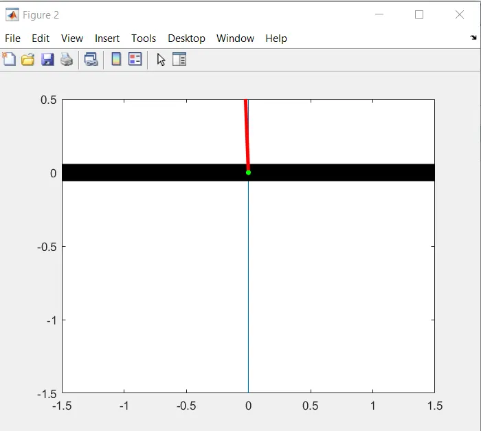
To create the animation of the pendulum we use the for loop mention the ct=1 because we calculate the result for the 500 position .for loop operating 500 times program for the for-end loop are as follow

• ct=1; initial count 1
• for i=1:length(result(:,1)) for loop initial condition wrt to I .
• x0=0; stating co-ordinate of x
• y0=0; stating co-ordinate of y
• x1=1*sin(result(i,1)); final co-ordinate of x
• y1=-1*cos(result(i,1)); final co-ordinate of y
• figure(2)
• plot([0,0],[-1.5,0.5]) fix vertical line
• hold on to showing result in single plot
• plot([-1.5,1.5],[0,0],'LineWidth',15,'Color','black') fixed support
• hold on
• plot([x0 x1],[y0 y1],'LineWidth',3,'Color','r') position of the pendulum length
• hold on
• axis ([-1.5 1.5 -1.5 0.5]) assign the axis of plot
• plot(x0,y0,'marker','.','MarkerSize',15,'Color','g') fix position of the pendulum
• plot(x1,y1,'marker','.','MarkerSize',60,'Color','g') free position of the pendulum ball
• M(ct)=getframe(gcf); capture the image data in one frame
• ct=ct+1; count incress by 1after every for loop
• hold off
• end ending with end command

8.Video file of out put

To creating the video of the output animation we write the following program

• movie(M) is usedto creat a film o f the stord data
• VideoWriter("ode2pendulum.m",'Uncompressed AVI') command specifies the name of the file where the video is going to store
• open(Videofile) is used to open video file data
• writeVideo(Videofile,M) command is uses to create the video animation by using m file
• close(Videofile) used to close video file data

Output And Result

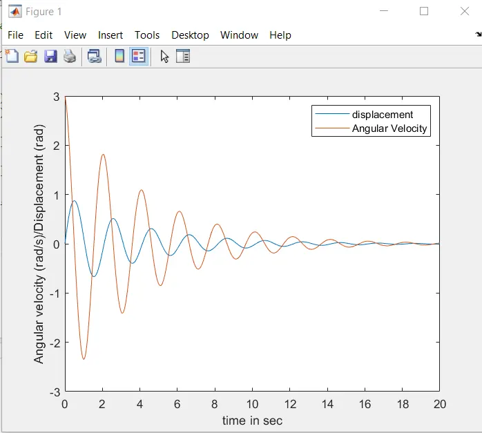
1 The out put obtained is graphical representation of Angular velocity (rad/s)/Displacement (rad) wrt time

• displacement stat from 0
• and Angular velocity startfrom 3 rad/sec
• after 20 sec both are become 0

2.Animation of the pendulum

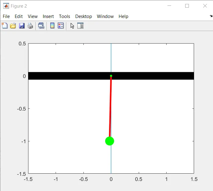
figure 2 show the animation of the pendulam

3.You tube link for an animation of the pendulum

https://youtu.be/QA1dgnia_ks

Errors and Output

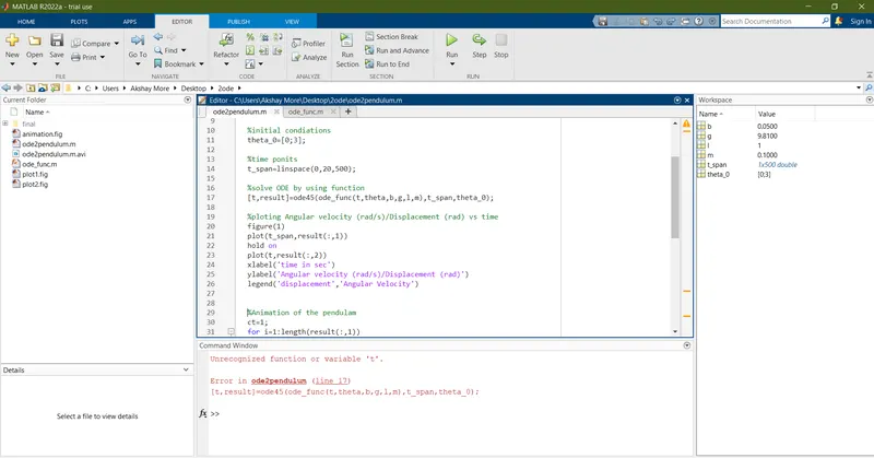
when devloping the program facing lots of errors and mistake here i am showing 2 errors

Error 1 missing the (-)minus sign

in final position of pendulum in y direction in for loop is y1=-1*cos(result(i,1)) but by mistakely i write y1=1*cos(result(i,1)) missing the minus sign

my program is running put position of pendulam was not showing correctly as show in fig

to overcome this mistake reading the program codding and correct the mistake

Error2 In ode 45 directly define the ode function not define the variable (t,theta) thats why program not running to overcome this error watching the video lecture and correct the my mistake

[t,result]=ode45(ode_func(t,theta,b,g,l,m),t_span,theta_0);

[t,result]=ode45(@(t,theta) ode_func(t,theta,b,g,l,m),t_span,theta_0);