Week 3 - Solving second order ODEs

%a program to solve second order diffretial equation 

clear all 
close all
clc

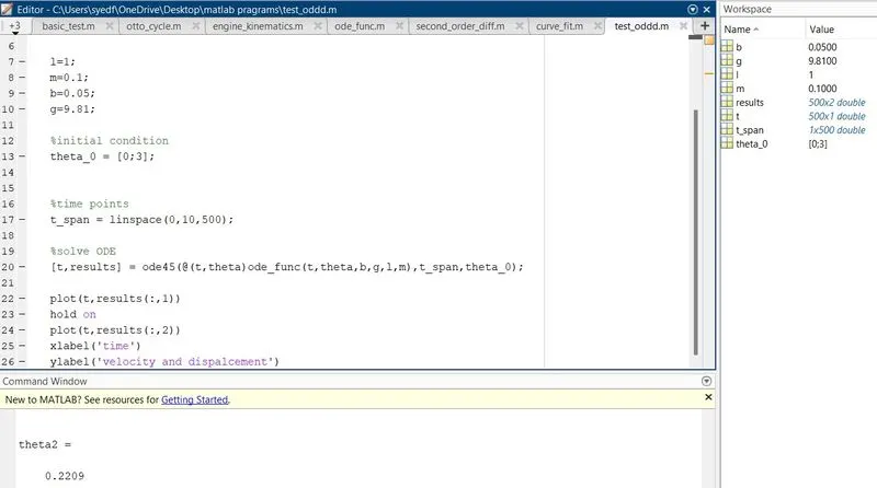
l=1;
m=0.1;
b=0.05;
g=9.81;

%initial condition
theta_0 = [0;3];


%time points
t_span = linspace(0,10,500);

%solve ODE
[t,results] = ode45(@(t,theta)ode_func(t,theta,b,g,l,m),t_span,theta_0);

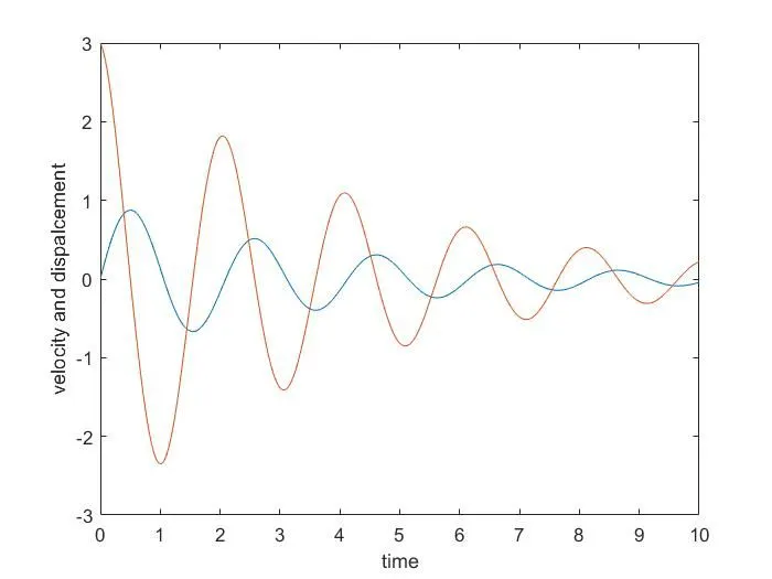
plot(t,results(:,1))
hold on 
plot(t,results(:,2))
xlabel('time')
ylabel('velocity and dispalcement')

Explanation :-

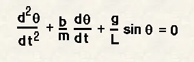
in the above equation

where, g = gravity in m/s2

L = length of the pendulum in m

m = mass of the ball in kg

b=damping coefficient

and given data is

L=1 metre

m=1 kg

b=0.05

g=9.81 m/s2

Simulate the motion between 0-20 sec, for angular displacement=0,angular velocity=3 rad/sec at time t=0.

after this

the initial conditions are

theta_0 = [0;3]

here in above there are two first ODE

ie,one is for displacement and another is for velocity

then time points

ie,

t_span=linspace(0,10,500);

and then solve ODE

[t,results] = ode45(@(t,theta),ode_func(t,theta,b,g,l,m),t_span,theta_0)

where ode45 is an inbulit function in matlab and defining ode45ie, (t,theta) and then defining a function(t,theta,b,g,l,m)

To use funtion defination the below programm is used

function [dtheta_dt]=ode_func(t,theta,b,g,l,m)
 theta1=theta(1)
 theta2=theta(2)
 dtheta1_dt=theta2;
 dtheta2_dt=-(b/m)*theta2-(g/l)*sin(theta1);
 dtheta_dt=[dtheta1_dt;dtheta2_dt];
end

and then plotting the (t,results of all rows and first column index and all rows and second column index)

ie,plot( t,results(:,1)) and (t,results(:,2))

Now to animate the motion of the simple pendulum

clear all
close all
clc


b=0.05;
g=9.81;
l=1;
m=0.1;

%initial condition
 theta_0=[0;3];

%time points
 t_span=linspace(0,10,500);

%solve ODE
 [t,results]=ode45(@(t,theta)ode_func(t,theta,b,g,l,m),t_span,theta_0);


plot(t,results(:,1))
hold on
plot(t,results(:,2))
ylabel('displacment,Velocity')
xlabel('time')
grid on
hold off

 ctr=1;
for i=1:length(results(:,1))
    x0=0;
    y0=0;
    x1=l*sin(results(i,1));
    y1=-l*cos(results(i,1));
    
    figure(2)
    plot([-0.5,0.5],[0 0],'linewidth',5,'color','r');
    line([x0 x1],[y0 y1],'linewidth',3,'color','g');
    hold on;

    plot(x1,y1,'o','markers',18,'markerfacecolor','b');
    axis([-1 1 -2 0.5]);
    hold off  
    grid on 
    M(ctr)=getframe(gcf);
    ctr=ctr+1;
end
%to creat movie
  movie(M)
  videofile = VideoWriter('pendulum_osilations.avi','uncompressed AVI');
  open(videofile)
  writeVideo(videofile,M)
  close(videofile)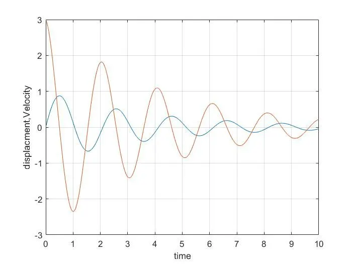

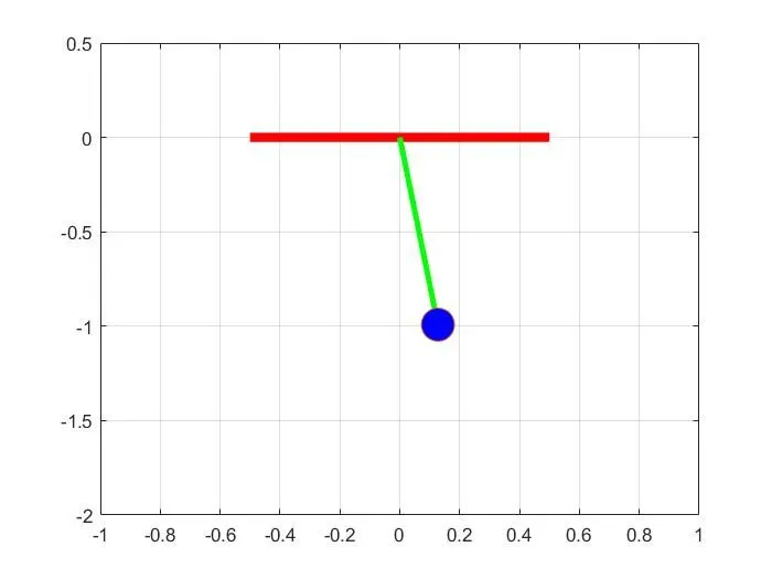
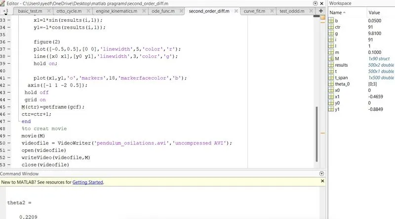
You tube link for an animation :-https://youtu.be/3JT6W0yFMV4

Explanation :- The above code shows how to animate the simple pendulum

as we know one end that is fixed end is called as 0,0 origin ie,x0=0 and y0=0

and then x1 and y1 can be x1=l*sin(results(i,1));
y1=-l*cos(results(i,1));

and then plotting [x0 x1] and [y0 y1]

and then using the markers command

basically marker command is nothing but making a mark of the given ie,0 it will creat a circle and if we use 's' square will be created

plot(x1,y1,'o','markers',18,'markerfacecolor','b');

basically it means plotting x1,y1 with a ball "o" with markers command and with a size of 18 and with a color of blue with a command "markerfacecolor"

and then to creat a video file

movie(M)
videofile = VideoWriter('pendulum_osilations.avi','uncompressed AVI');
open(videofile)
writeVideo(videofile,M)
close(videofile)

You tube link for an animation :-https://youtu.be/3JT6W0yFMV4

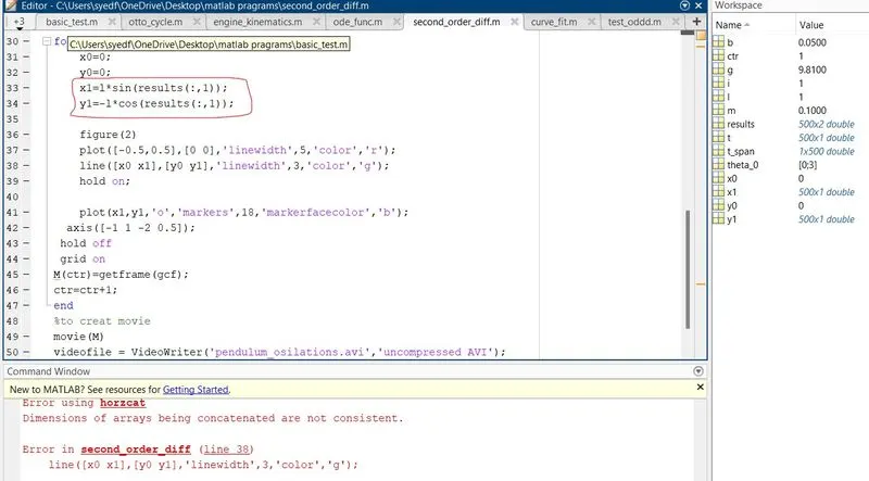
error i got is insted of "i" i had used "The colon"

and even to creat a video file i had used "videowriter" instead of capital "VideoWriter"