Week 3 - Solving second order ODEs

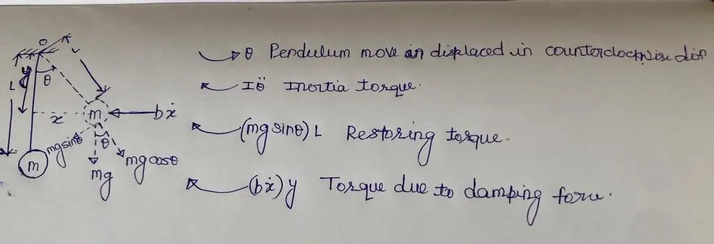
Let `theta`=angular displacement of the pendulum in a counterclockwise direction.

then after restoring torques will act on the pendulum to come back to its original position.

`Iddottheta`=Inertia torque in a clockwise direction

where I=moment of inertia of mass m about a fixed point through which pendulum oscillates.

`I=mL^2`

`(mgsintheta)L`=torque in a clockwise direction due to gravitational force mg.

`(bdotx)L=(bdotthetaL)L=bdotthetaL^2`=torque in a clockwise direction due to damping force`

Now apply equilibrium method,

`Iddottheta+bL^2dottheta+mgLsintheta=0`

`mL^2ddottheta+bL^2dottheta+mgLsintheta=0`

`ddottheta+b/mdottheta+g/Lsintheta=0`

`(d^2theta)/(dt^2)+b/m(d theta)/(dt)+g/Lsintheta=0`----------(1)

Since `theta`(displacement) is very small. so we can write `sintheta=theta`. hence equation (1) becomes

`(d^2theta)/(dt^2)+b/m(d theta)/(dt)+g/Ltheta=0`----------(2)

Equation (1) is the second-order ordinary differential equation, representing the change in pendulum position `(theta)` with time (t).

Here,

b=Damping Coefficient=0.05

m=Mass of ball=1kg

g=Acceleration due to gravity=9.81 m/s^2

L=Length of pendulum=1m

Analytical solution:

`(d^2theta)/(dt^2)+b/m(d theta)/(dt)+g/Ltheta=0`

Auxiliary equation: `alpha^2+b/malpha+g/L=0`

the analytical solution of the above equation has two roots `alpha_1 and alpha_2`

`alpha_(1,2)=(-b/m+-sqrt((b/m)^2-4g/L))/2`

`alpha_(1,2)=-b/(2m)+-sqrt((b/(2m))^2-g/L`

Analytic solution will be,

Displacement

`theta=Ae^(alpha_1t)+Be^(alpha_2t)`

Velocity

`dottheta=Aalpha_1e^(alpha_1t)+Balpha_2e^(alpha_2t)`

Numerical Solution using MATLAB

`(d^2theta)/(dt^2)+b/m(d theta)/(dt)+g/Lsintheta=0`

First, we transform second order ode into two first-order odes.

Assume, `theta=theta_1`

`(d theta)/dt=(d theta_1)/dt=theta_2`----------(A)

`(d^2theta)/dt^2=(d theta_2)/dt`

`(d(theta_2))/(dt)+b/mtheta_2+g/Lsintheta_1=0`

`(d theta_2)/(dt)=-b/mtheta_2-g/Lsintheta_1`----------(B)

Now second order ode(equation 1) has transformed into two first odes (equation A and B)

Now we transform equation A and B in Matrix form

`d/dt[[theta_1],[theta_2]]=[[theta_2],[-b/mtheta_2-g/Lsintheta_1]]`

`d/dt[[displacement],[velocity]]=[[theta_2],[-b/mtheta_2-g/Lsintheta_1]]`

`(d theta)/dt=[[theta_2],[-b/mtheta_2-g/Lsintheta_1]]`

Here `theta`is the column vector of displacement and velocity.

MATLAB Main Code

clear all
close all
clc

%% input 
b=0.05;     % damping coefficient
m=1;        % mass of ball (kg)
g=9.81;     % acceleration due to gravity (m/s^2)
L=1;        % pendulum length (m)

%% initial condition
theta_0=[0;3];      % initial angular displacement =0 and initial angular velocity=3 rad/s

%% time points
time_span=linspace(0,20,500);

%% ode45 solver
[t,displacement_velocity]= ode45(@(t,theta) ode_function_code(t,theta,b,m,g,L),time_span,theta_0);

%% plot
figure(1)
plot(t,displacement_velocity(:,1))
hold on
plot(t,displacement_velocity(:,2))
xlabel('Time')
ylabel('Angular displacement & Angular velocity')
legend('Angular displacement','Angular velocity')
grid on

%% writting a for loop to make animation
ct=1;
for i=1:length(displacement_velocity(:,1))
    x0=0; y0=0;
    x1=L*sin(displacement_velocity(i,1)); y1=-L*cos(displacement_velocity(i,1)); 
    figure(2)
    plot([-1 1],[0 0],'linewidth',3)
    hold on
    plot([x0 x1],[y0 y1],'linewidth',3)
    hold on
    plot(x1,y1,'o','markersize',20,'markerfacecolor','y')
    axis([-2 2 -2 2])
    pause(0.03)
    hold off
    M(ct)=getframe(gcf);
    ct=ct+1;
end

%% converting the animation  into movie
movie(M)
videofile=VideoWriter('pendulum_oscillation.avi','Uncompressed AVI');
open(videofile)
writeVideo(videofile,M)
close(videofile)

MATLAB Function Code

function [dtheta_dt]=ode_function_code(t,theta,b,m,g,L)
theta1=theta(1);
theta2=theta(2);
dtheta1_dt=theta2;
dtheta2_dt=-(b/m)*theta2-(g/L)*sin(theta1);
dtheta_dt=[dtheta1_dt;dtheta2_dt];

end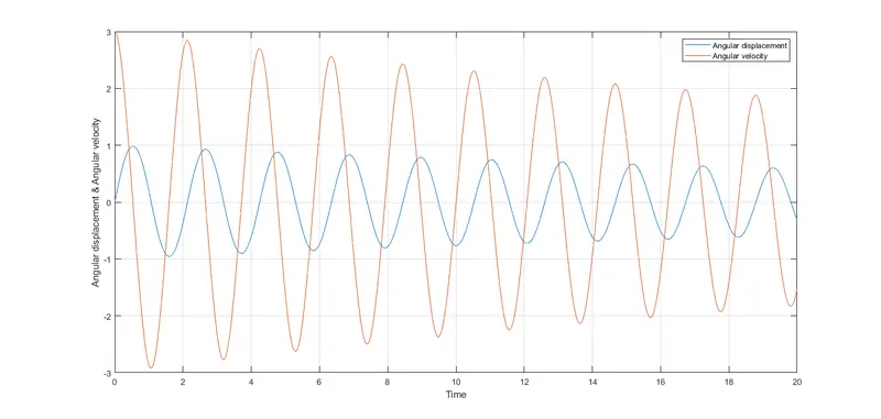

Animation link

https://drive.google.com/file/d/1UfwPOtn5kHeonmiLfy0p9p_gqqTV7vY5/view?usp=sharing