Aim- To write a program that solves the following ODE. This ODE represents the equation of motion of a simple pendulum with damping

In Engineering, ODE is used to describe the transient behavior of a system. A simple example is a pendulum

The way the pendulum moves depends on Newton's second law. When this law is written down, we get a second-order Ordinary Differential Equation that describes the position of the "ball" w.r.t time.

Similarly, there are hundreds of ODEs that describe key phenomena and if you have the ability to solve these equations then you will be able to simulate any of these systems.

This ODE represents the equation of motion of a simple pendulum with damping

In the above equation,

g = gravity in m/s2,

L = length of the pendulum in m,

m = mass of the ball in kg,

b=damping coefficient.

Given Conditions:-

L=1 metre,

m=1 kg,

b=0.05.

g=9.81 m/s2.

Time span= 0-20 sec

for angular displacement=0,angular velocity=3 rad/sec at time t=0.

Functions used-

ode45

ode_func calculations:-

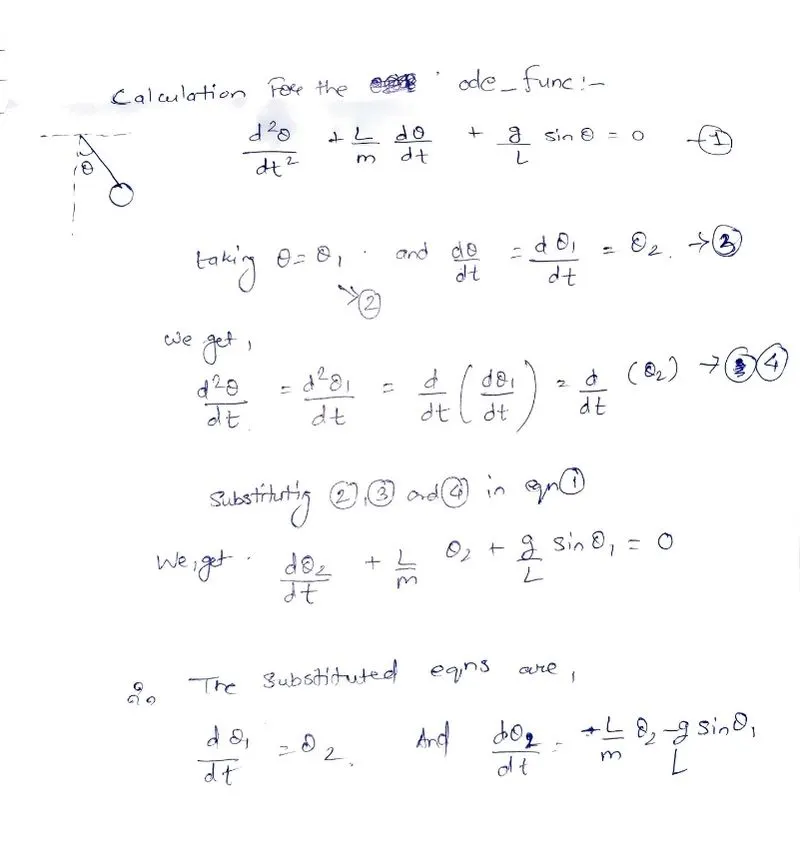
The program for the function used to simplify and calculate the ode is attached below;

function [dtheta_dt] = ode_func(t,theta,b,g,L,m)

theta1 = theta(1)
theta2 = theta(2)
dtheta1_dt = theta2;
dtheta2_dt = -(b/m)*theta2 - (g/L)*sin(theta1);
dtheta_dt= [dtheta1_dt; dtheta2_dt];
end

Main Code- Code for solving the ODE representing the equation of motion of a simple pendulum with damping.

The function called ("ode_func")in the main code is attached above.

%Program to solve the ODE equation of motion of a simple pendulum with
%damping


clear all
close all
clc

% Given values
b=0.05;
g=9.81;
L=1;
m=0.1;

%Initial condition
theta_0= [0;3];                 %[angular dipacement;angular velocity]

%time points
t_span = linspace(0,20,500);

%solve ODE
[t,results] = ode45(@(t,theta) ode_func(t,theta,b,g,L,m),t_span, theta_0);

figure(1)
plot(t,results(:,1),'Color','r')
hold on
plot (t,results(:,2),'Color','b')
ylabel('Angular displacement(red)/Angular velocity(blue)')
xlabel('time')

% plotting animation of pendulum
ct=1;
figure(2)

for i=1:length(t_span)
    x0=0;
    y0=0;
    x1= L*sind(results(i,1));
    y1= -L*cosd(results(i,1));           %along angular displacement

    plot([x0 x1], [y0 y1],'linewidth',3,'Color','r')
    hold on
    plot(x1,y1,'Marker','o','MarkerSize',20,'MarkerFaceColor','b','MarkerEdgeColor','r')
    axis([-0.1 0.15 -1.2 0.15])
    pause(0.03)
hold off
    M(ct)=getframe(gcf);
    ct=ct+1;
end


movie(M)
videofile = VideoWriter('ode_pendulum.avi', 'Uncompressed AVI');
 open(videofile)
 writeVideo(videofile,M)
 close(videofile)

Here, for y1= -L*cosd(results(i, 1)); the Negative sign is used for inverting the pendulum to obtain the desired output.

Output- The output animation video link of the motion of the simple pendulum with damping is attached below:-

https://drive.google.com/file/d/1LoUh9-geiTmC761IyIZGfStKoBQp47XN/view?usp=sharing

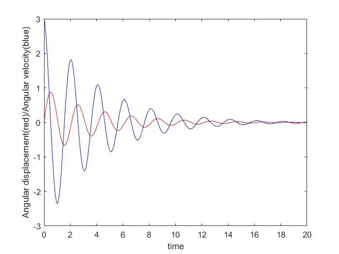
Output 2-

• The figure shows the plot for angular displacement and angular velocity with respect to time.

Errors occurred-

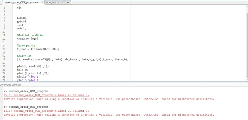
Here, in line 20 , plot(t,results9(:,1))

Typing error was made hence the following invalid expression error was shown in the command window.

It was rectified and the plot ran successfully.

Conclusion- The program to solve the second-order ODE for simple pendulum motion with damping was executed successfully and the animation link was attached to the report. Errors faced were rectified.