Week 3 - Solving second order ODEs

Aim: The main aim of the challenge is to solve the ODE which represent the equation of motion of a simple pendulum with damping.

Objective of the challenge: To write a program to solve the following ODE which represent the equation of motion of a simple pendulum with damping and create an animated video of the output obtains by solving the the ODE.

Theory: 

The motion of the simple pendulum is the basic example of the simple harmonic motion,as in the figure shown below it consist of the bob and the massless string. The movement of the pendulum depends on newtons second law. When this law is written down, a second order ordinary differential equation is formed that describe the position of the pendulum at starting and end position with respoect to time through angle theta as shown in the figure below 

equation of the motion is 

in the above equation,

L = length of the pendulum in meter 

m = mass of the ball in kg 

b = damping coefficient 

g = gravity in m/s^2

theta = angle made by the pendulum in too and pro motion 

since the given equation is in the second order differential equation first we will convert it into first order in order to solve ODE

let theta = theta1

dtheta1_dt = theta2 

Inputs:

l = 1;

m = 1;

b = 0.05;

g = 9.81;

angular displacement = 0;

angular velocity = 5; at time t=0

code:

% Program to simulate the motion of the simple pendulum.
clear all 
close all 
clc 
 
%inputs 
b = 0.05;             %damping coefficient%
g = 9.81;             %gravity%
l = 1;                %length of the pendulum in meter%
m = 1;              %mass of the ball in kg%

%initial condition 
theta_0 = [0;3];

%time points 
t_span = linspace(0,20,500);

%solve ODE
[t, results] = ode45(@(t,theta) ode_func(t, theta, b, g, l, m), t_span, theta_0);

plot(t,results(:,1))
hold on
plot(t,results(:,2))
xlabel('time')
ylabel('results')

% iteration using for loop command to create the animation movie of simple pendulum 
ct = 1
theta_1 = results(:,1);

for i= 1:length(results(:,1))
    theta_2 = theta_1(i);

    % initial co-ordinates 
    x_start = 0;
    y_start = 0;

    x_end = l*sin(theta_2);
    y_end = -l*cos(theta_2);

    %ploting for the movie animation
    figure(2)
    %movement of the pendulum as a base
    plot([-1,1],[0,0],'linewidth',3,'color','r')
    hold on
    %ploting of pendulum movement with respect to the cordinates
    line([x_start, x_end],[y_start, y_end],'linewidth',3,'color','b')
    %bob of the pendulum at both ends of the cordinates 
    plot(x_end,y_end,'marker','o','markerSize',28,'markerfacecolor','black')
    axis([-2 2 -2 2])
    pause(0.03)
    hold off
    M(ct) = getframe(gcf);
    ct = ct+1;
end 

%creating the movie from the above capture frames
movie(M)
videofile = VideoWriter('simple_pendulum.avi','Uncompressed AVI')
open(videofile);
writeVideo(videofile,M);
close(videofile)

Code for the function program:

function  [dtheta_dt] = ode_func(t,theta,b,g,l,m)
theta1 = theta(1)
theta2 = theta(2)
dtheta1_dt = theta2 
dtheta2_dt = -(b/m)*theta2 - (g/l)*sin(theta1);
dtheta_dt = [dtheta1_dt;dtheta2_dt];
end 

detail explanation of each steps of the program:

first start the program with the clear all, close all and clc which is very important as clear all removes the data from the workspace and freeing up system memory and close all delete the current figure or the specified figure and clc clears all the inputs and outputs from the command window display giving you a clean screen.

1) In the first step start applying the inputs and the intial condition of the simple pendulum 

2) then the program is written to solve the ODE in which matlab inbuilt function (ode45) is used with constant theta, t and another function is used, which is defined seperately in function program.

3)in the next step result of solved ODE is plotted w.r.t time using plot command.

4)now the iteration of the cordinates is applied using for loop to create the animation.

5)then plot command is used to plot the pendulum base,string and using the cordinates plotting  pendulum bob.

6)in the next step movie command is used to create the animated video of the oscillating pendulum then videowriter command is to assign the video format for this project.avi was used as a format.then the open command was used to open the videofile. writevideo command is used to write the video with plot frames. finally close command was used to close the video file.

output:

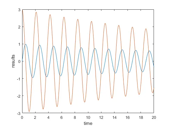
Explaination of the plot graph:

with respest to time ,the result i.e angular velocity and angular displacement variation take place in the pendulum motion with the damping coefficient  as shown in the graph above 

various error i faced during the programm as follows :

in program during for loop iteration i done the mistake in writing theta2 instead of theta_2 when i was assigning the variable theta_2 = theta_1(i)

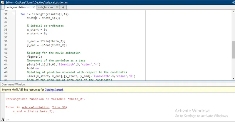
 Then step taken to overcome this error, i made it correct by writing it correct theta_2 and the function runs fine.

2) typing mistake in plotting bob of the pendulum where i done mistake in typing Markesize, '0' instead of 'o' and faced the error 

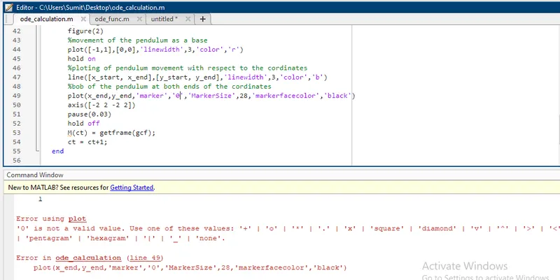
The step taken to overcome this problem is i corrected the mistake by writing markersize and 'o' instead of '0'

3) the pendulum start oscilaating in an inverted direction in an animated video as i have bymistake change the sign of the cordinated instead of '-' sign to sin i wrote the '-' sign to cos and pendulum strart oscilating in the inverted position.

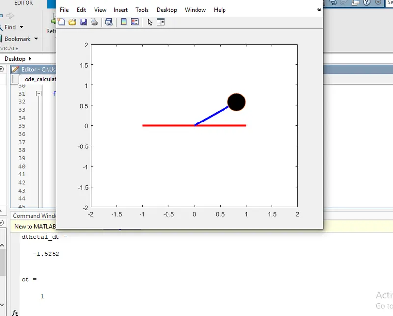
By taking the measure of this error i just change the sign to the cordinates, 

the final cordinate , x_end =-l *sin(theta_2) changed to l*sin*(theta_2)and y_end = 1*cos(theta_2) changed to y_end = -1*cos(theta_2)

Conclusion:

the simulation of the transient behaviour of a simple pendulum is successfully created by the matlab program

Animated video:- 

here is the link of the video of the animation i got for this project

https://youtu.be/9fcImVWydwo