Week 3 - Solving second order ODEs
*Report of second order ODE’s in MATLAB : Simple Pendulum
*challenge_skill lync-ganesh katkar
Aim : Solve the animation of the pendulum using the equation of second order differential ode’s.
Objective : Program to find and animate solutions for single pendulum oscillation using ODE’s in the matlab program.
Problem statements: To write a code that solves second order ODE for simulating the pendulum motion and to create the animation of the pendulum.
Body of the content:
Solution :
A pendulum is a body suspended from a fixed point so that it can swing back and forth under the influence of gravity. The time interval of a pendulum’s complete back-and-forth movement is constant.
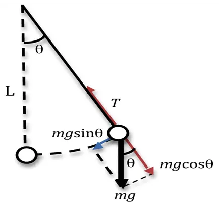
Where,
b = damping coefficient
m = mass of the bob kg,
g = acceleration due to gravity m/
l = length of the string m.
Started the matlab program
First of all type the variable to save and run the program.
% Second order ODE’s simple Pendulum
clear all
close all
clc
Then defined the input
% Input values
b = 0.05;
g = 9.81;
l = 1;
m = 1;
There are 2 types of order ODE to solve the ODE’s system,one for velocity & second for displacement.
The initial displacement of the pendulum is 0 and the initial velocity is 3m/sec.
% initial condition
theta_0 = [0;3];
Integrat ODE’s system to solve.t_span is a time array. It will go from 0 to 25 second. It has 700 values.
% time points
t_span = linspace(0,20,600);
% solve ODE
[t,results] = ode45(@(t,theta) ode_func(t,theta,b,g,l,m),t_span,theta_0);
…ode45 is an inbuilt solver in matlab program.
…(t,theta) are the main inputs of ode, t & theta are dependent & independent variables of ode system.
…ode_func is (t,theta,b,g,l,m). we will pass these input parameters.
…t_span is the time to integrate the time array.
…theta_0 are the initial condition is corresponding.
ode_func(t,theta,b,g,l,m)
function [dtheta_dt] = ode_func(t,theta,b,g,l,m)
theta1 = theta(1)
theta2 = theta(2)
dtheta1_dt = theta2;
dtheta2_dt = -(b/m)*theta2 - (g/1)*sin(theta1);
d𝜃1/dt = 𝜃2
/dt = -(b/m)𝜃2 – (g/l)sin𝜃1
It is combine in an array.
dtheta_dt = [dtheta1_dt; dtheta2_dt];
figure(1)
plot(t,results(:,1))
hold on
plot(t,results(:,2))
ylabel('plot')
xlabel('time')
after we execute this program we get this plot.
Here are two curves after executing the program,the first curve indicates displacement and the second curve indicates velocity.
The displacement starts from 0 and the velocity starts from 3.5m/s.
for i = 1:length(t)clc
x1 = 0;
y1 = 0;
x2 = 1*sin(results(i,1))
y2 = -1*cos(results(i,1));
x3 = -1;
y3 = 0;
x4 = 1;
y4 = 0;
figure(2)
plot([x3 x4],[y3 y4],'LineWidth',7,'Color','r')
hold on
plot([x1 x2],[y1 y2],'LineWidth',5,'Color','g')
hold on
plot(x2,y2,'o','MarkerSize',25,'MarkerFaceColor','y')
hold off
axis([-2 2 -2 2]);
pause(0.02);
M(ct)= getframe(gcf);
ct = ct+1
end
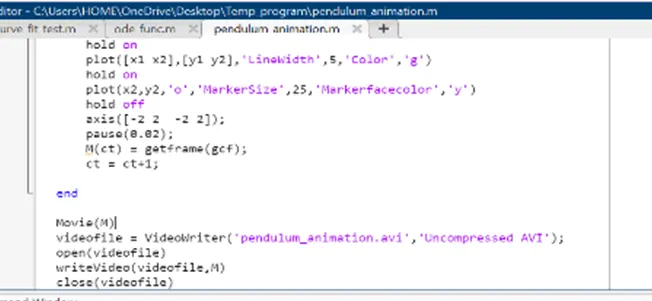
…We are getting the frame that is in array called ‘M’
Then type,
Movie(M)
videofile = VideoWriter('pendulum_animation.avi','Uncompressed AVI');
open(videofile)
Once we have creat this file ,just open it,type
Open(videofile)
Write(videofile,M)
Close(videofile)
Now after going to execute the program its an a animation,and its play the movie
Here is the link for watch an animation
Error detected while coading : Animation is not saved in the movie file when the middle (m) of the movie is kept short to make an animated movie,so it is saved as Movie(M) to save an animated movie.
conclusion: finally we getting an movie animation for second order differential equation ODE’s pendulum with the help of matlab.