Week 3 - Solving second order ODEs

Aim: Write a program in python to simulate the motion of a pendulum.

Objectives :

Write a program to solve the following ODE.
Write a program in python to simulate the motion of a pendulum.

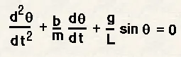
Theory: ODE is used to describe the transient behaviour of a system. In the above equation,

g = gravity (m/s^2)

L=length of pendulum in m

m=mass of ball in kg

b= damping coefficient

Given:

L= 1m

m= 1kg

b=0.05

g=9.81m/s^2

Simulate the motion between 0-20 s

• for angular dispacement = 0
• angular velocity = 3 rad/s
• at time t = 0

Program :

import numpy as np
from scipy.integrate import odeint
import math
import matplotlib.pyplot as plt


#function that returns dtheta/dt

def function(theta,t,b,g,l,m):
    theta1=theta[0]
    theta2=theta[1]
    dtheta1_dt=theta2
    dtheta2_dt=-(b/m)*theta2-(g/l)*math.sin(theta1)
    dtheta_dt=[dtheta1_dt,dtheta2_dt]
    return dtheta_dt


b=0.05
g=9.81
l=1
m=1

#initial condition
theta_0=[0,3]

#time points
t=np.linspace(0,20,200)

#solve ode
theta=odeint(function,theta_0,t,args=(b,g,l,m))

#plot result
plt.plot(t,theta[:,0],'g-',label=r'$\frac{d\theta_1}{dt}=\theta2$')
plt.plot(t,theta[:,1],'b--',label=r'$\frac{d\theta2}{dt}=-\frac{b}{m}\theta_2-\frac{g}{l}sin\theta_1$')
plt.xlabel('Plot')
plt.ylabel('Time')
plt.legend()
plt.savefig('Output.png')
plt.show()

#animation
ct=1

x0=0
y0=0

for i in theta[:,0]:

    x1=(1*math.sin(i))
    y1=(-1*math.cos(i))

    filename='test%05d.png'%ct 
    ct=ct+1

    plt.figure()
    plt.plot([-1,1],[0,0],"black",linewidth=10)
    plt.plot([x0,x1],[y0,y1],"red")
    plt.plot(x1,y1,'o',markersize=20)
    plt.xlim([-1.5,1.5])
    plt.ylim([-1.5,1.0])
    plt.savefig(filename)

Steps used for coding:

• Import module numpy and np, scipy.integrate, import odeint for second ODE, mathe and plots matplotlib.
• Define function that returns the value of dtheta/dt.
• Initialize the input values b,g,l & m.
• Define initial condition for theta; 0 and 3 rad/s.
• Use np.linspace for creating numerical sequence.
• Solve ODE using odeint command.
• Plot resultusing plt.plot command.
• For animation, use for loop.

Results:

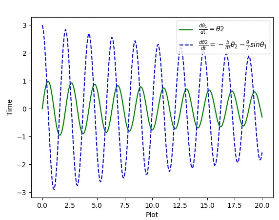
https://drive.google.com/file/d/1ps-8s85dn-m-VUlGKyu-Ev4hK_vtT89l/view?usp=sharing

Conclusion:

The above graph shows the variation of angular velocity and angular dispacement, and it changes over time due to damping effect.