Week 3 - Solving second order ODEs

Aim: - Write a program to simulate the motion of simple pendulum

Objectives: - 1) To write a matlab program using ode45 solver to solve second order differential equation

2) To plot a graph of velocity and displacement variation w.r.t time

3) To create animation of motion of simple pendulum.

Introduction to Ordinary Differential Equation

Ordinary differential equation abbreviated as ODE is the most important concept in mathematical, social, and natural sciences. Mathematical descriptions of change use differentials and derivatives. Various differentials, derivatives, and functions become related via equations, such that a differential equation is a result that describes dynamically changing phenomena, evolution, and variation.

ODE is an equation having variables and a derivative of the dependent variable with reference to the independent variable. ODE in real life includes its use to calculate the movement or flow of electricity, to study the to and fro motion of a pendulum, to check the growth of diseases, mathematical models involving population growth, in radioactive decay studies and many more. In this particular challenge, the motion of a simple pendulum has been simulated with the use of Matlab.

Simple pendulum

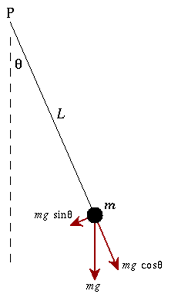
A simple pendulum consists of a mass m hanging from a string of length L and fixed at a pivot point P. when displaced to an initial angle and released, the pendulum will swing back and forth with periodic motion. The equation of motion for the pendulum can be obtained using Newton’s second law for rotational systems.

Governing equation

The motion of pendulum is governed by second-order differential equation. Mathematically it is represented as:-

Where: - θ is the angle made by the movable link with vertical axis

b is damping coefficient

l is the length of string

m is mass of bob

g is acceleration due to gravity

t is time

In order to solve this equation in Matlab and find the variation of θ w.r.t time we first break this second order differential equation into two first order differential equation.

Let θ = θ₁

Putting the values in equation 1 we get

Equation 4 and 5 represents two first ODE representing velocity and displacement respectively.

Matlab code for simulation of pendulum motion

close all
clear all
clc

%input variables
b = 0.1;                                   % damping coefficient
l = 1;                                     % length of string (m)
g = 9.81;                                  % acceleration due to gravity (m/s^2)
m = 1;                                     % mass of bob (kg)


% initial condition 
theta_0 = [0;5];

% time span
t_span = linspace(0,20,500);

% solve ode
[t,results] = ode45(@(t,theta)ode_func(t,theta,b,g,l,m),t_span,theta_0);

figure(1)                                  % figure plots the graph of velocity and displacement
plot(t,results(:,1))
hold on
plot(t,results(:,2))
ylabel('plot')
xlabel('time')


%%ANIMATION
X0=0;
Y0=0;

ct=1;                                     %counter actually represents each and every frame
for i=1:length(t)
    X1=l*sin(results(i,1));
    Y1=-l*cos(results(i,1));
    
    figure(2)
    plot([-1 1],[0 0],'linewidth',6,'color','g');
    axis([-2  2 -2 2]);
    line([X0 X1],[Y0 Y1],'linewidth',2,'color','b');
    hold on;
    plot(X0,Y0,'O','markersize',3,'markerfacecolor','y');
    plot(X1,Y1,'O','markersize',20,'markerfacecolor','r');
    title('Damping of simple pendulum');
    legend('support rod','length of pendulum','fixed point','bob of pendulum');
    grid on;
    hold off;
    M(ct)=getframe(gcf);
    ct=ct+1;
end


movie(M);
videofile = VideoWriter('simple_pendulum','Uncompressed AVI');
open(videofile);
writeVideo(videofile,M);
close(videofile);

    

Code for ode function

function[dtheta_dt] = ode_func(t,theta,b,g,l,m)
theta1 = theta(1)
theta2 = theta(2)
dtheta1_dt = theta2;
dtheta2_dt = -(b/m)*theta2-(g/l)*sin(theta1);
dtheta_dt = [dtheta1_dt;dtheta2_dt];
end

Stepwise explanation of code: -

• Program starts with clear all, close all, clc
• Length of rod, mass of bob, damping coefficient and acceleration due to gravity is taken as input variables.
• To provide the initial condition of the pendulum a column vector is created with 0 and 5 as value of displacement and velocity respectively.
• Time span of 20 sec is created using linspace command.
• To solve the differential equation ode45 solver is used.
• Ode45 is an inbuilt solver in Matlab that is used to solve ordinary differential equation or partial differential equation using numerical technique. The syntax for the solver is as follows.

[T,Y] = ode45(odefun,tspan,y0)

• t and results are the output vectors. t is the column vector for time points and results stores the solution array.

• Ode_func is the function that is created to store the two first order differential equation. The two ode are stored in a column vector named dtheta_dt and then passed to ode45 solver for integration.
• Figure (1) is created to plot the velocity and displacement variation w.r.t time.
• Figure (2) is created to store different images of pendulum.
• getframe command is used to capture figures as movie frame.
• Movie(M) command play recorded movie frames.
• videoWriter command is used to write video files.
• writeVideo command is used to write video data to file.

Results and discussion: -

The plot of velocity and displacement w.r.t time has been shown below.

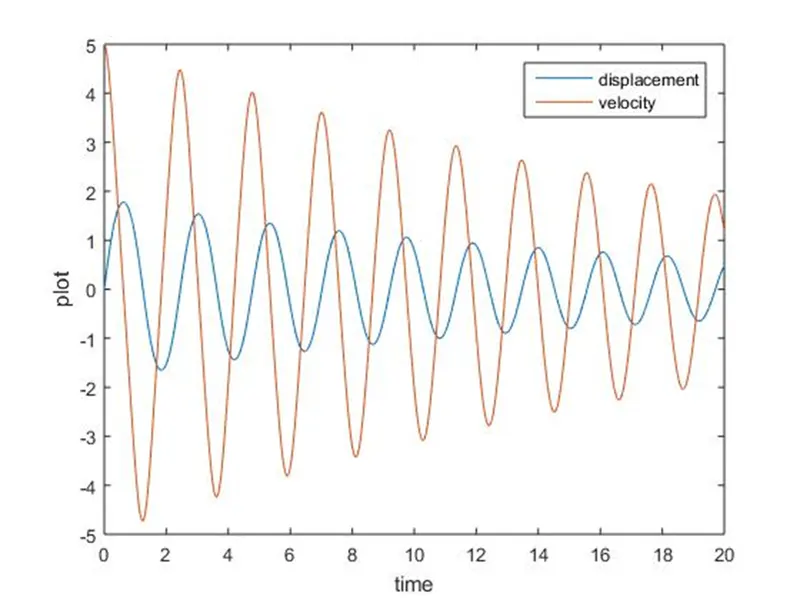
• The plot shows the variation of velocity and displacement over a time span of 20 sec.
• Pendulum starts with the initial velocity of 5 rad/s and reduces to 1.168 rad/s after 20 sec with the damping coefficient of 0.1

Errors: -

Some of the errors were made while writing the program

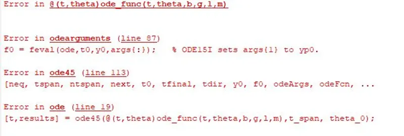
The error was in ode45 syntax. The error was resolved by passing the sufficient parameters in ode_func.

There was typing mistake in the above line. The error was resolved by correcting videofile.M to videofile,M.

Animation: -

Conclusions: -

• A matlab code was written which successfully simulated the motion of simple pendulum.
• The efficacy of ode45 solver in solving the non stiff differential equation was studied.
• The displacement and velocity graph was plotted.
• An animation was created showing the motion of simple pendulum.