Week 3 - Solving second order ODEs

1 ) AIM : To create animation of simple pendulum using matlab.

2 ) GOVERNING EQUATION :

`d^2theta/dt^2 + (b/m)(d theta)/dt +g/Lsintheta = 0`

here,

g = gravity in m/s,

L = length of the pendulum in m,

m = mass of the ball in kg,

b = damping coefficient.

the above equation is 2nd order differential equation .

3 ) OBJECTIVE :

• The objective is to solve 2nd order differential equation .

here we are having case of simple pendulum. we are converting 2nd order equation into 1st order and writing programe for it.

• here we are also making animation video of simple pendulum and uploading it on youtube.

4 ) BODY :

• The equation of pendulum is 2nd order differential equation. we are converting 2nd order differential equation into 1st order differential equation.
• Then we use function command to create funtion .
• used marker command to highlight ball ,support and pndulum.

here we have created function.

function [ dtheta_dt] = ode_func(t,theta,b,g,l,m)
theta1 = theta(1)
theta2 = theta(2)
dtheta1_dt = theta2;
dtheta2_dt = -(b/m)*theta2 - (g/l)*sin(theta1);
dtheta_dt = [ dtheta1_dt ; dtheta2_dt];
end

now we are using above function and creating another program to calculate simple pendulum and making animation of simple pendulum.

clear all
close all
clc

%inputs

b = 0.05; %damping
g = 9.81; % gravity
l = 1 ; % length of pendulum
m = 1; % mass of pendulum

% initial conditions
theta_0 = [0;3];  % initial dosplace is zero and initial velocitycis 5


% time points 
t_span = linspace(0,20,500);

% solve ODE

[t,results] = ode45(@(t,theta) ode_func(t,theta,b,g,l,m),t_span, theta_0);

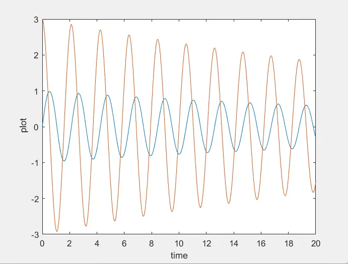
plot (t,results(:,1))
hold on
plot(t,results(:,2))
xlabel('time')
ylabel(' plot')

x0 = 0;
y0 =0 ;

ct=1;

for i = 1 : length(t)

    x1 = l*sin(results(i,1));
    y1 = -l*cos(results(i,1));


figure (2)
plot ([-2 2] , [0 0] ,'linewidth' ,8 ,'color' , 'g');
axis([-2 2 -2 2 ]);
line([x0 x1] , [y0 y1],'linewidth',2,'color', 'b');
hold on;
plot (x0,y0,'o','markersize',3,'markerfacecolor','y');
plot (x1,y1,'o' , 'markersize',20,'markerfacecolor','r');
title ('Damping of simple pendulum');
legend('support rod','length of pendulum','fixed support','Bob of pendulum');
grid on;
hold off;
M(ct) = getframe(gcf);
ct = ct+1;
end

movie(M)
videofile = VideoWriter('ode_main.avi','Uncompressed AVI')
open(videofile)
writeVideo(videofile,M)
close(videofile)

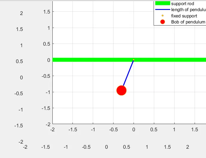
Here is the link of animation of simple pendulum.

https://youtu.be/09Zh2jsJu5s

5 ) CONCLUSION :

we can conclude that ,we can see in image that waves are dying at very slow rate which is due to low damping coefficient and small time fram.