Project 2 - Rankine cycle Simulator

  AIM  : 

• To create Rankine cycle simulator using matlab .
• To develop program which calculate state point.
• To plot T-S and H-S curves .

THEORY :

The rankine cycle is the fundamental operating cycle of all power plants where an operating fluid is continuously evapourated and condensed . The selection of operating fluid depends mainly on the available temperature range.

                  

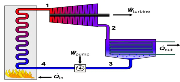
The rankine cycle is operated in following ways :-

Process 1-2  Isentropic Expansion :

The vapour is expanded in the turbine , thus producing work which may be converted to electricity.Here the mechanical energy is converted into electrical energy.

work produce by turbine is given by :

`W_T = (h1-h2)`

Process 2-3 Constant pressure heat Rejection :

The expanded vapour is then passed through a condenser where heat is rejected at constant pressure and the steam is converted into water again.This liquid is again pumped to the boiler.

`Q_r = m(h2-h3)`

process 3-4  Isentropic compression :

The water enters the pump in saturated state.Then the liquid is compressed isentropically untill it meets the boiler pressure .

Work done by the pump is given by :

`W_p = m(h3-h4)`

Process 4-1 Constant Pressure heat addition :

The water enters into the boiler as compressed and leaves as superheated from the boiler . Thus the phase changes from liquid to vapour .

The heat supplied by the boiler is 

`Q_b = m(h1-h4)`

Here we are taking mass flow rate m = 1 

• The efficiency is given by:

`eta_(th) = W_n/Q_1 = (W_T - W_P)/Q_1`

• Applying the steady state flow Energy Equation (SFEE) to all the process , neglacting the friction losses and changes in kinetic and potential energy,

     Q1 = h1 -h4

     Wt = h1-h2

     Q2 = h2 - h3 

     Wp = h4 - h3

•   The capacity of the steam plant is often expressed interms of Steam Rate (SR) or Specific Steam Consumption (SSC).

   `S.S.C = 3600/W_n (Kg)/(KWh)`

Required inputs :

Turbine Inlet temperature = 400° C

Turbine Inlet Pressure = 30 bars

Turbine Outlet Pressure = 0.05 bars = Condenser Inlet Pressure

                   MATLAB CODE                       

clear all
close all
clc

fprintf('      SIMULATOR OF RANKINE CYCLE\n')
fprintf('1-2 Isentropic Expanssionin the turbine\n')
fprintf( '2-3 constant pressure Heat Rejection by the condenser\n ' )
fprintf('3-1 Isentropic compression in the pump\n')
fprintf('4-1 constant pressure Heat addition by the Boiler\n')


%inputs
 p1 = input ('Enter the pressure at turbine inlet (in bar): ');
 t1 = input ('Enter the Temperature at the turbine inlet (in degree celsius): ');
 p2 = input ('Enter the pressure at the Condenser (in bar): ');
 disp('   Results')

 %getting cp and cv values from xsteam
 %cp and cv assumed to not change with temperature to make problem simple

 % for vapour
 high_cpV = XSteam('CpV_p',p1);
 low_cpV = XSteam('CpV_p',p2);
 high_cvV = XSteam('cvV_p',p1);
 low_cvV  = XSteam('cvV_p',p2);

 % for liquid
 high_cpL = XSteam('CpL_p',p1);
 low_cpL = XSteam('CpL_p',p2);
 high_cvL = XSteam('cvL_p',p1);
 low_cvL  = XSteam('cvL_p',p2);
 

 %getting important parameters from Xsteam
 %for high pressure

 t1s = XSteam('Tsat_p',p1);
 s1g = XSteam('sV_p',p1);
 s1f = XSteam('SL_p',p1);
 s1fg = s1g - s1f ;
 h1f = XSteam('hL_p',p1);
 h1g = XSteam('hV_p',p1);
 h1fg = h1g - h1f;

 % for low pressure

 t2s = XSteam('Tsat_p',p2);
 s2g = XSteam('sV_p',p2);
 s2f = XSteam('SL_p',p2);
 s2fg = s2g - s2f ;
 h2f = XSteam('hL_p',p2);
 h2g = XSteam('hV_p',p2);
 h2fg = h2g - h2f;


 %% state point 1

 disp('At state point 1: ')
 fprintf( 'p1 is : %f bar\n',p1)
 fprintf(' t1 is : %f Deg celcius\n',t1);

 h1 = XSteam('h_pt',p1,t1);
 fprintf('h1 is : %f KJ/Kg\n',h1);

 s1 = XSteam('s_pt',p1,t1);
 fprintf('s1 is : %f KJ/KgK\n',s1)


 %% state point 2

 disp( 'At state point 2 : ')
 fprintf('p2 is : %f bar\n',p2)

 s2=s1;
 fprintf('s2 is : %f kj/kgk\n',s2);

 %predicting location of point 2 in T-S

 if (s2<=s2g)
     x2 = (s2-s2f)/(s2fg);  %deyness fraction at state point 2
 else
     x2 = 1 ;
 end

 fprintf('x2 is : %f \n' ,x2);

 %calculating t2 for superheate or wet or dry wherever it lies 
 if (x2<1)
     t2=t2s;
 else

     %t2 cal by s2=s2g+low_cpV*(log(t2/t2s))

     t2 =(t2s+273.15)*exp((s2-s2g)/low_cpV);  % in superheated region
     t2 = t2 - 273.15;

 end

 fprintf('t2 is : %f Deg celcius\n',t2)

 if(x2<1)
     h2 = h2f + x2*h2fg;
 else
     h2 = h2g+ low_cpV*(t2-t2s);
 end

 fprintf('h2 is : %f kj/kg\n',h2)

 %% state point 3

 % assuming no subcooling assumed

 disp(' At state point 3: ');

 p3 = p2;
 fprintf('p3 is : %f bar\n',p3)

 v3 = XSteam('vL_p', p3);

 t3 = t2s ; % no subcooling assumed
 fprintf('t3 is : %f Deg celcius\n',t3)

 h3 = h2f ;
 fprintf('h3 is : %f kj/kg\n',h3);

 s3=s2f;
 fprintf('s3 is : %f kj/kgk\n',s3);


 %% state point 4
 disp('At state point 4 : ')
 p4 = p1;
 fprintf('p4 is : %f bar\n',p4);

 s4 =s3;
 fprintf('s4 is : %f kj/kg\n',s4);

 wp = v3* (p4-p3)*100;
 h4 = wp +h3 ;
 fprintf(' h4 is : %f kj/kg\n',h4);

 % to calculate t4 s4=s3=sf1-high_cpL*ln(t1s/t4)
 term = exp((s1f-s4)/high_cpL); 
 t4 = t1s/term;
 fprintf('t4 is : %f DEg celcius \n',t4);


 %% calcuylation of work done ,heat ,SSC and efficiency 

 wt = h1-h2;
 fprintf('work by turbine is : %f kj/kg\n', wt);
 fprintf('work by compressor is : %f kj/kg\n', wp);

 wnet = wt - wp;
 fprintf('net work done is : %f kj/kg\n', wnet);

 Qin = h1 - h4; % heat supplied

 eff_thermal = (wnet/Qin)*100 ; % efficiency
a = sprintf('Thermal efficiency is : %f%%\n', eff_thermal); 
disp(a)
SSC = 3600/wt;    % specific steam consuption
fprintf('S.S.C  is : %f kj/kwh\n', SSC);

%% Calculation for plotting liquid and vapour lines
%
% <>
%
temp = linspace(1,373,500);
for i = 1:length(temp)
    H_L(i) = XSteam('hL_T',temp(i));
    H_V(i) = XSteam('hV_T',temp(i));
    S_L(i) = XSteam('sL_T',temp(i));
    S_V(i) = XSteam('sV_T',temp(i));

end

%% ploting T-S and H-S diagram
   

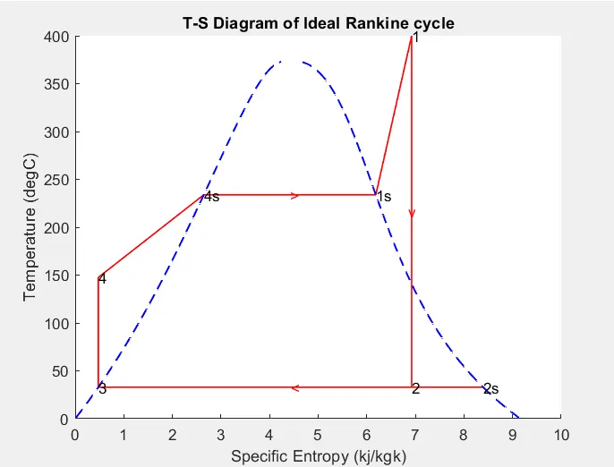
figure(1)
hold on
plot ([s1 s2],[t1 t2],'r','LineWidth',1)
text(s1,t1,'1')
text(s2,t2,'2')
plot ([s2 s2g],[t2 t2s],'r','LineWidth',1)
text(s2g,t2s,'2s')
plot ([s2g s3],[t2s t3],'r','LineWidth',1)
text(s3,t3,'3')
plot ([s3 s4],[t3 t4],'r','LineWidth',1)
text(s4,t4,'4')
plot ([s4 s1f],[t4 t1s],'r','LineWidth',1)
text(s1f,t1s,'4s')
plot ([s1f s1g],[t1s t1s],'r','LineWidth',1)
text(s1g,t1s,'1s')
plot ( [s1g s1 ], [t1s t1],'r','LineWidth',1)

plot(S_L , temp, 'b' , 'LineStyle','--','LineWidth',1)
plot(S_V , temp, 'b' , 'LineStyle','--','LineWidth',1)
%marking direction 

text(s1,(t1+t2)/2,'v','HorizontalAlignment','center','Color','r')
text((s2g+s2f)/2,t3,'<','color','r')
text(s3,(t3+t4)/2,t3,'v','HorizontalAlignment','center','Color','r')
text((s1f+s1g)/2,t1s,'>','Color','r')
title('T-S Diagram of Ideal Rankine cycle')
xlabel('Specific Entropy (kj/kgk)')
ylabel('Temperature (degC)')

%%

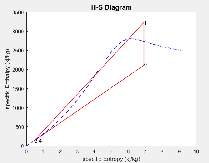
figure (2)
hold on
plot([s1 s2],[h1 h2],'r','LineWidth',1)
text(s1,h1,'1')
plot([s2 s3],[h2 h3],'r','LineWidth',1)
text(s2,h2,'2')
plot([s3 s4],[h3 h4],'r','LineWidth',1)
text(s3,h3,'3,4')
plot([s4 s1],[h4 h1],'r','LineWidth',1)
%text(s4,h4,'4')
plot(S_L , H_L, 'b' , 'LineStyle','--','LineWidth',1)
plot(S_V , H_V, 'b' , 'LineStyle','--','LineWidth',1)
title('H-S Diagram','FontSize',13)
xlabel('specific Entropy (kj/kg)')
ylabel('specific Enthalpy (kj/kg)')

    COMMAND WINDOW OUTPUT : 

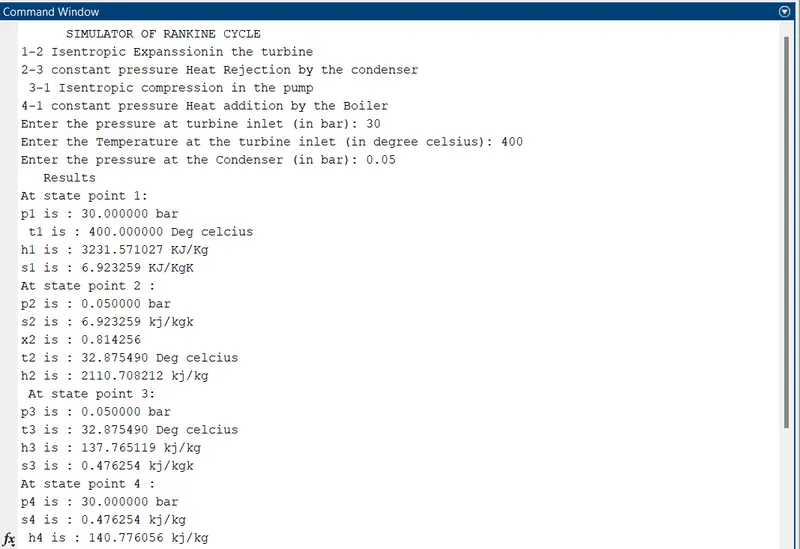
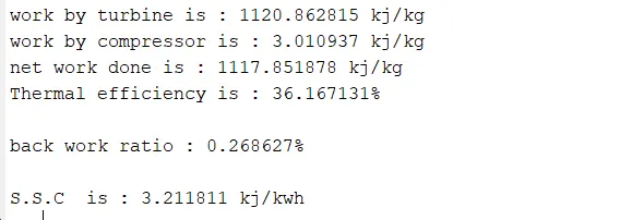
          WORKSPACE OUTPUT :

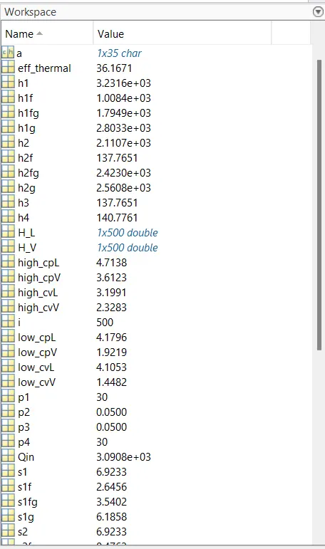
       T-S  Diagram 

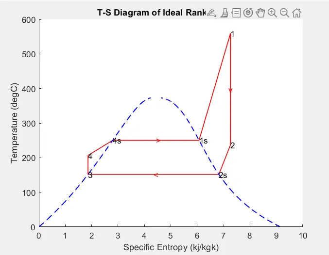
For superheated graph will be :

    H-S    Diagram :

 CONCLUSION :

• Efficiency of rankine cycle increases in superheating.
• By changing input data we can see various output.

    REFERENCE :

• skill - lync projects 
• chrome