Week 3 - Solving second order ODEs
The following submission include code for damped pendulum motion
0. Solving given objective ODE in challenge and plotting Amplitude vs time
1. Solving ODE derived via Free Body Diagram method and plotting Amplitude vs time
2. Animating the motion of pendulum as given in objective
COMPLETE CODE inclue objective 0. objective 1. objective 2.
%Skill lync- week 2-MATLAB Basic-Bhavin Chaudhary date 7/03/2022 to 10/03/2022
%Solving Second order differential equation
%We will consider all the vibrating system linear. Hence differential is linear
%objective
%0. Generate code to solve given objective ODE Equation & plot amplitude/velocity vs time plot
%1. Generate code for pendulum damped oscillating motion and plot amplitude/velocity vs time plot
%2. We will animate the pendulum motion

%0. code to plot given second-ODE for pendulum motion
syms m %mass of hanging bob in Kg
syms l %length of pendulum in m
syms b %damping coefficient in N.s/m
syms g %gravity constant of earth in m/s^2
syms t_i %starting or initial time in s
syms t_f %ending or final time in s
syms I % incremental value or number of fragments of given time frame
syms t_span %span of time frame
syms i_c %initial condition of oscillation
disp('0. CODE TO SOLVE SECOND ORDER DIFFERENTIAL EQUATION OF PENDULUM DAMPED MOTION')
l=input('enter the value of length of pendulum in m=')
m=input('enter the value of mass of bob in Kg=')
b=input('enter the value of damping coefficient=')
g=input('enter the value of gravity in m/s^2=')
v=input('enter the maximum velocity of pendulum in rad/s=')
t_i=input('enter the initial value of time in seconds=')
t_f=input('enter the final value of time in seconds=')
I=input('enter the increment or fragments of time span=')
t_span=linspace(t_i,t_f,I);
i_c=[0;v]; %defines initial condition of input matrix
%note the first row is theta and second row is angular velocity in above initial condition
t_span=linspace(t_i,t_f,I); %this defines the time span for which we need solution
%below ode operator solves ordinary differential equation which is an inbuild MATLAB solver
%here results is a matrix Mx2 matrix with two column
[t, results]=ode45(@(t,theta) w2_mb_function_ode_damped_pendulum_motion(t,theta,b,m,l,g),t_span, i_c);
hold on
%here result(:,m) is extraction of matrix from results matrix
%Note the first column of result matrix is theta and second column is angular velocity
plot(t,results(:,1),'color','r') %plots angular displacementi.e. theta with respect to time
plot(t,results(:,2),'color','b') %plots angulat velocit i.e. dtheta/dt wrt time
plot([0 t_f],[0 0],'color','k') %plots the y=0 line
title('Skill-Lync:equation-A:Plot for Viscous under-Damped pendulum system')
xlabel('time in seconds')
ylabel('Angular displacement in rad/ Angular velocity in rad/s')
legend('Angular Displacement','Angular Velocity')
grid on

%1. Code to plot amplitude/velocity vs time for oscillating pendulum motion using equation of motion derived via free body diagram
syms theta %angular displacement
syms m %mass of hanging ball
syms g %gravity constant
syms L %length of pendulum system
syms Ct %damping coefficient
syms It %moment of inertia of pendulum system
syms Kt %torsional stifness
syms Cct%critical damping coefficient
syms eta%damping factor
syms omegan%natural frequency
syms v %maximum angular velocity
syms t_i %initial time
syms t_f %final time
syms I %increment or fragment of time span
syms t_span %time span
syms omegad %damping frequency
syms delta %logarithmic decrement of system
%code to solve the second order differential equation for basic viscous damping system
disp('1. CODE TO SOLVE SECOND ORDER DIFFERENTIAL EQUATION (Derived by FBD method) OF PENDULUM DAMPED MOTION')
m=input('enter the mass of hanging ball in Kg=')
L=input('enter the length of pendulum system in m=')
g=input('enter the value of gravity in m/s^2=')
Ct=input('enter the value of damping(equivalent damping)torsional coefficient=')
V=input('enter the maximum value of angular velocity in radian/s=')
t_i=input('enter the initial value of time in second=')
t_f=input('enter the final value of time in seconds=')
I=input('enter the increment fragments of time in number')
disp('Tortional inertia of system It')
It=m*L^2
disp('tortional stiffness of system Kt')
Kt=m*g*L
disp('nautral frequency of system omegan')
omegan=(Kt/It)^0.5
disp('Critical damping coefficient')
Cct=2*It*omegan
%the damping factor in damped oscillating system
disp('Damping factors')
eta=Ct/Cct
disp('damping frequency of system')
omegad=omegan*((1-(eta^2))^(-1/2))
disp('logarithmic decrement of amplitude of the system')
delta=(2*pi*eta)/((1-eta^2)^0.5)

%enter the initial condition vector
i_c=[0;V];
t_span=linspace(t_i,t_f,I);
[t, results]=ode45(@(t,theta) w2_mb_function_ode_viscous_damping_torsional(t,theta,Kt,It,Ct), t_span, i_c);
theta=results(:,1);
hold on
plot(t,results(:,1),'color','r')
plot(t,results(:,2),'color','b')
plot([0 t_f],[0 0],'color','k')
title('Skill-Lync:EQUATION-B:Plot for Viscous under-Damped pendulum system')
xlabel('time in seconds')
ylabel('Angular displacement in rad/ Angular velocity in rad/s')
legend('Angular Displacement','Angular Velocity')
grid on

%3. code to animate the pendulum motion
syms theta %angular displacement in radian
syms THETA %angular displacement in degree
syms m %mass of hanging ball
syms g %gravity constant
syms L %length of pendulum system
syms Ct %damping coefficient
syms It %moment of inertia of pendulum system
syms Kt %torsional stifness
syms Cct%critical damping coefficient
syms eta%damping factor
syms omegan%natural frequency
syms v %maximum angular velocity
syms t_i %initial time
syms t_f %final time
syms I %increment or fragment of time span
syms t_span %time span
syms omegad %damping frequency
syms delta %logarithmic decrement of system
syms x0 %initial abscissa of rope
syms y0 %initial ordinate of rope
syms x1 %final abscissa of rope
syms y1 %final ordinate of rope
%code to solve the second order differential equation for basic viscous damping system
disp('2. ANIMATION OF DAMPED PENDULUM MOTION')
m=input('enter the mass of hanging ball in Kg')
L=input('enter the length of pendulum system in m=')
g=input('enter the value of gravity in m/s^2=')
Ct=input('enter the value of damping(equivalent damping)torsional coefficient=')
V=input('enter the maximum value of angular velocity in radian/s=')
t_i=input('enter the initial value of time in second=')
t_f=input('enter the final value of time in seconds=')
I=input('enter the increment fragments of time in number')
disp('Tortional inertia of system It')
It=m*L^2
disp('tortional stiffness of system Kt')
Kt=m*g*L
disp('nautral frequency of system omegan')
omegan=(Kt/It)^0.5
disp('Critical damping coefficient')
Cct=2*It*omegan
%the damping factor in damped oscillating system
disp('Damping factors')
eta=Ct/Cct
disp('damping frequency of system')
omegad=omegan*((1-(eta^2))^(-1/2))
disp('logarithmic decrement of amplitude of the system')
delta=(2*pi*eta)/((1-eta^2)^0.5)

%enter the initial condition vector
i_c=[0;V];
t_span=linspace(t_i,t_f,I);
[t, results]=ode45(@(t,theta) w2_mb_function_ode_viscous_damping_torsional(t,theta,Kt,It,Ct), t_span, i_c);
%solution of angular displacement in radian
theta=results(:,1);
%solution of angular displacement converted into degree
THETA=(180/pi).*theta;
x0=0; %initial abscissa of rope
y0=0; %initial ordinate of rope
ct=1;
for i=1:length(THETA)
    T=THETA(i);
    x1=L*cosd(-90+T);
    y1=L*sind(-90+T);
    plot([x0 x1],[y0 y1],[x1 x1],[y1 y1],'-or','linewidth',3,'Markersize',20)
    title('skill-lync:equation B:free damped pendulum oscillatory motion')
    legend('rope','spherical bob')
    grid on
    axis([-1 1 -2 0])
    pause(0.000001)
    M(ct)=getframe(gcf)
    ct=ct+1;
end
movie(M)
videofile=VideoWriter('pendulum_free_damped_oscillation.avi','Uncompressed AVI');
open(videofile)
writeVideo(videofile,M)
close(videofile)
function[dtheta_dt]=w2_mb_function_ode_damped_pendulum_motion(t,theta,b,m,l,g)
theta1=theta(1);
theta2=theta(2);
dtheta1_dt=theta2;
dtheta2_dt=-((b/m)*theta2)-((g/l)*sin(theta1));
dtheta_dt=[dtheta1_dt;dtheta2_dt];


function[dtheta_dt]=w2_mb_function_ode_viscous_damping_torsional(t,theta,Kt,It,Ct)
theta1=theta(1);
theta2=theta(2);
dtheta1_dt=theta2;
dtheta2_dt=-((Ct/It)*theta2)-((Kt/It)*theta1);
dtheta_dt=[dtheta1_dt;dtheta2_dt];
end
OBJECTIVE 0.
OUTPUT
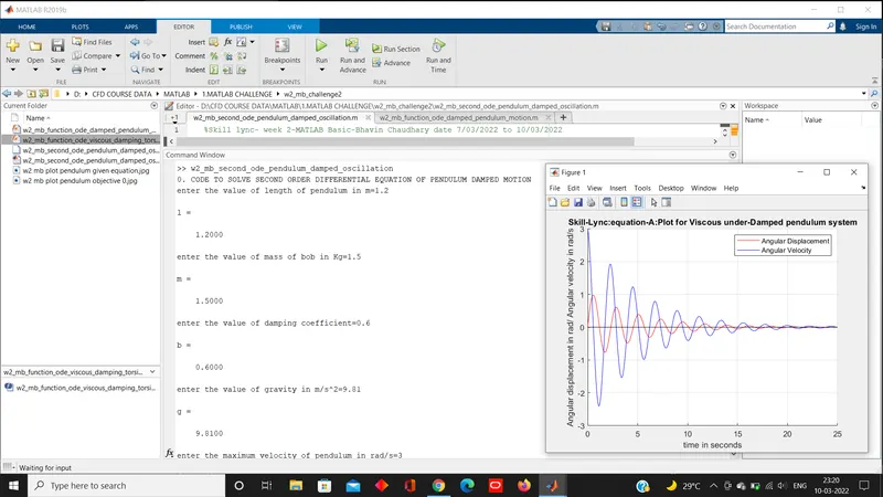
>> w2_mb_second_ode_pendulum_damped_oscillation
0. CODE TO SOLVE SECOND ORDER DIFFERENTIAL EQUATION OF PENDULUM DAMPED MOTION
enter the value of length of pendulum in m=1.2
l =
1.2000
enter the value of mass of bob in Kg=1.5
m =
1.5000
enter the value of damping coefficient=0.6
b =
0.6000
enter the value of gravity in m/s^2=9.81
g =
9.8100
enter the maximum velocity of pendulum in rad/s=3
v =
3
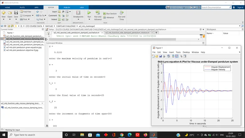
enter the initial value of time in seconds=0
t_i =
0
enter the final value of time in seconds=25
t_f =
25
enter the increment or fragments of time span=300
I =
300
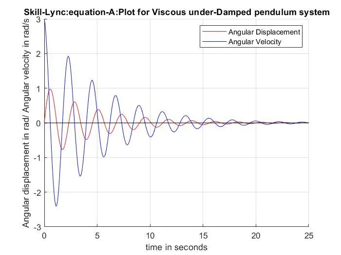
OBJECTIVE 0.
SREENSHOT
OBJECTIVE 1.
OUTPUT
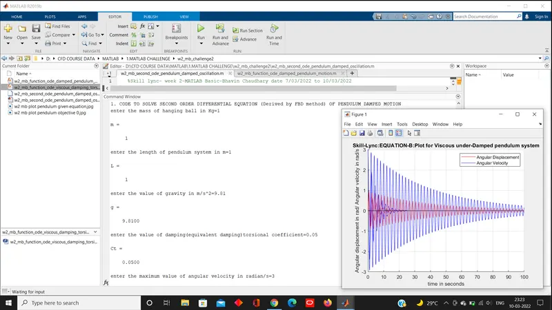
1. CODE TO SOLVE SECOND ORDER DIFFERENTIAL EQUATION (Derived by FBD method) OF PENDULUM DAMPED MOTION
enter the mass of hanging ball in Kg=1
m =
1
enter the length of pendulum system in m=1
L =
1
enter the value of gravity in m/s^2=9.81
g =
9.8100
enter the value of damping(equivalent damping)torsional coefficient=0.05
Ct =
0.0500
enter the maximum value of angular velocity in radian/s=3
V =
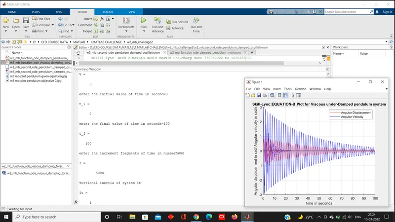
3
enter the initial value of time in second=0
t_i =
0
enter the final value of time in seconds=100
t_f =
100
enter the increment fragments of time in number5000
I =
5000
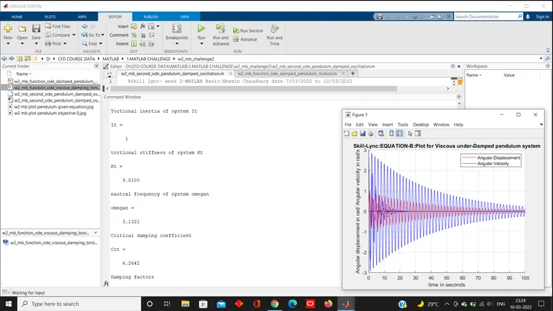
Tortional inertia of system It
It =
1
tortional stiffness of system Kt
Kt =
9.8100
nautral frequency of system omegan
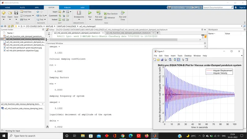
omegan =
3.1321
Critical damping coefficient
Cct =
6.2642
Damping factors
eta =
0.0080
damping frequency of system
omegad =
3.1322
logarithmic decrement of amplitude of the system
delta =
0.0502
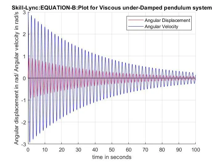
OBJECTIVE 1.
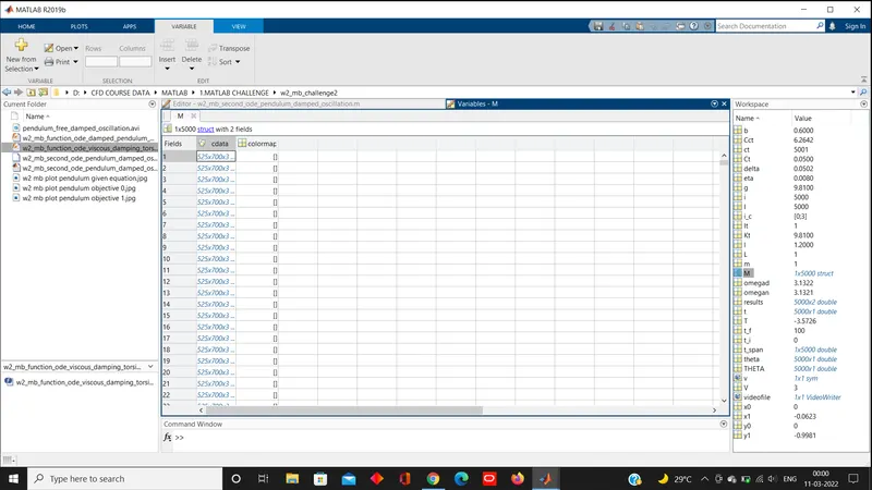
SCREENSHOT
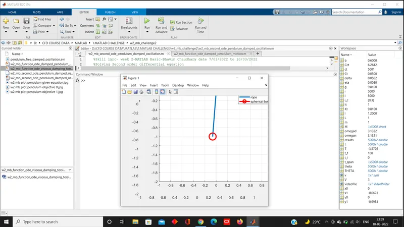
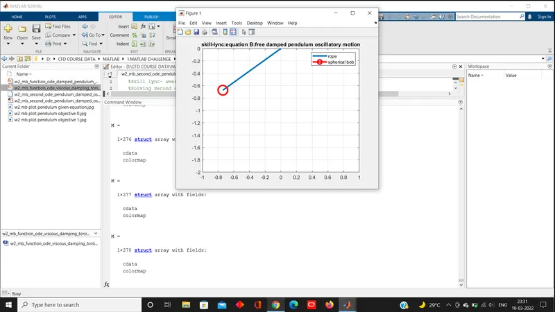
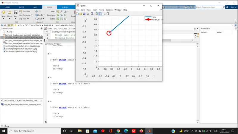
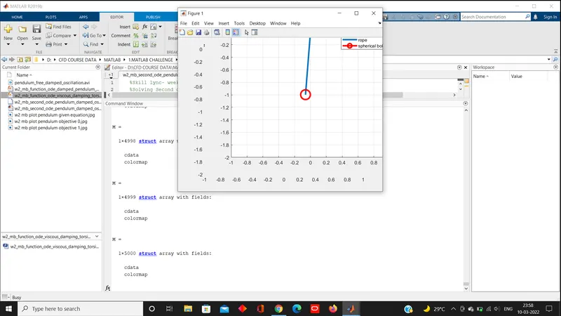
OBJECTIVE 2.
OUTPUT
enter the mass of hanging ball in Kg=1
m =
1
enter the length of pendulum system in m=1
L =
1
enter the value of gravity in m/s^2=9.81
g =
9.8100
enter the value of damping(equivalent damping)torsional coefficient=0.05
Ct =
0.0500
enter the maximum value of angular velocity in radian/s=3
V =
3
enter the initial value of time in second=0
t_i =
0
enter the final value of time in seconds=100
t_f =
100
enter the increment fragments of time in number5000
I =
5000
Tortional inertia of system It
It =
1
tortional stiffness of system Kt
Kt =
9.8100
nautral frequency of system omegan
omegan =
3.1321
Critical damping coefficient
Cct =
6.2642
Damping factors
eta =
0.0080
damping frequency of system
omegad =
3.1322
logarithmic decrement of amplitude of the system
delta =
0.0502
SCREENSHOT
YOUTUBE VIDEO LINK