Week 3 - Solving second order ODEs

Objective: To see a simulation of the simple pendulum by solving second-order ordinary differential equations using Python.

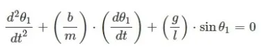
Theory: This ODE represents the equation of motion of a simple pendulum with damping

In the above equation,

g = gravity in m/s2,

L = length of the pendulum in m,

m = mass of the ball in kg,

b=damping coefficient.

Now, we cannot solve second order ODE in python so, for that, we convert this second order ODE into the first-order ODE which shown as follows:-

Let, say θ=θ1

Then equation(1) tends to

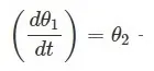
And, if θ1 change with respect to time we can say that

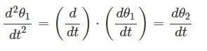
Also, we can say that

Now,by substituting equation(3) & (4) in equation (2),we get

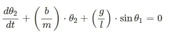
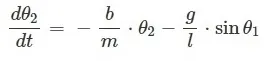
By, using equation (3) & (4) which is of first-order we will simulate simple pendulum by using Python.

Code:

In the following code, first, we have import all the necessary modules that are needed to solve ode after that we have allocated the useful parameter.

After then we have defined the ode function, in which we have created the matrix for dtheta_dt so, that we can calculate displacement and velocity. After that,

we will call this function in the odeint line so that we can solve ode equation.

And then we plotted time versus displacement and time versus velocity in the same figure using subplot command.

Also, we have created the animation of the pendulum for the time span.

close all
clear all
clc

b=0.05;
g=9.81;
l=1;
m=1;

% initial condition
theta_0=[0;3];

% time points
t_span=linspace(0,20,200);

%solve ODE
[t,results]=ode45(@(t,theta)ode_function(theta,b,g,l,m),t_span,theta_0);

figure(1)
plot(t,results(:,1))
hold on
plot(t,results(:,2))
xlabel('time')
ylabel('angular velocity')
title('motion of pendulam')
legend('displacement','angular velocity')


% for loop creation
ct=1;
for i=1:length(t_span)
    %coordinates
     x = l*sin(results(i,1));
     y = -l*cos(results(i,1));
     
     %plotting of the bob motion.
     figure(2)
     plot([-3 3],[0 0],'linewidth',2,'color','b');
     hold on
     plot([0 x],[0 y],'linewidth',3,'color','g');
     plot(x,y,'o','markers',15,'MarkerFaceColor','y');
     axis([-3 3 -2 2]);
     grid on
     pause(0.03)
     M(ct)=getframe(gcf);
     ct=ct+1;
     hold off
end
     
% animation
movie(M)
videofile=VideoWriter('simple_pendulam.avi','uncompressed AVI');
open(videofile)
writeVideo(videofile,M)
close(videofile)

    
   
 

Function

function [dtheta_dt]=ode_function(theta,b,g,l,m)
theta1=theta(1);
theta2=theta(2);
dtheta1_dt=theta2;
dtheta2_dt=-(b/m)*theta2-(g/l)*sin(theta1);
dtheta_dt=[dtheta1_dt;dtheta2_dt];
end

Output

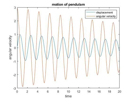
Observation: By observing the above figure its quite clear that as time increases displacement and velocity decrease, because of the damping effect.

Animation video:

https://drive.google.com/file/d/1U81AykmotWb2809KskzEIB4O3INsgIbI/view?usp=sharing