Week 3 - Solving second order ODEs

Aim: To write a progame in Matlab that will simulate the pendulum motion.

Objective:

• First objective is to write a program that solves the 2 order ODE.
• To write a program in Matlab that will simulate the pendulum motion.
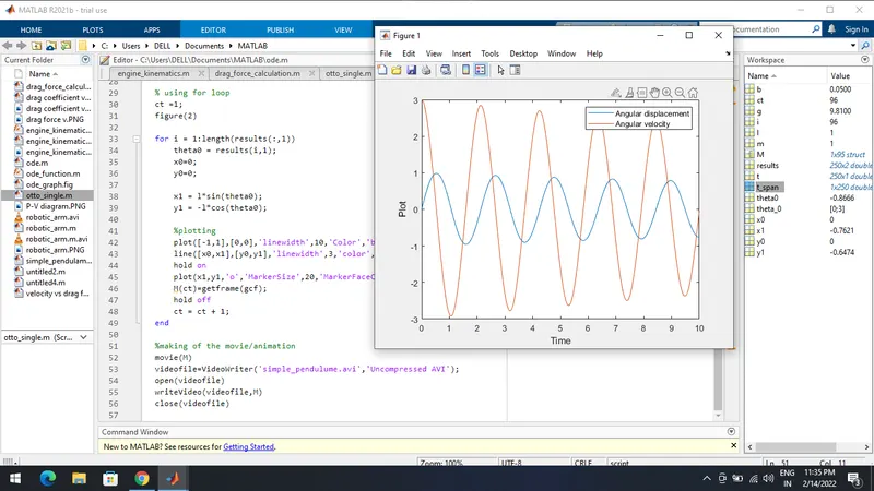
• To plot the graph of displacement and velocity v/s time and animate the motion of bob.

Governing Equation:

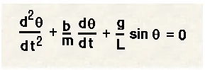
where:

b = damping coefficient

m = mass of the bob (kg)

g = acceleration due to gravity (m/s^2)

l = length of the string in (m)

Theory:

A simple pendulum consisits of a mass (m) hanging from a string of length (L) and fixed at a pivot point
(p). when displace to an initial angle and released, the pendulum will swing back and forth with periodic motion.

Code Explanation:

• Programing language used MATLAB online
• starting the program by using comments
• Providing the input variables like (L= 1 meter,m=1kg, b=0.005,g=9.81m/s^2)
• Providing the values for theta-O & using linspace command for time span=0 to for 250 values
• Solving the ODE by use of the predefined function and for the ODE formula
• Now plot the graph for the displacement & velocity w.r.t to time
• Now using 'for' command for iterating the values of the desired variable
• Assuming the values for x0,y0=0
• Providing the eqn for the x1,y1 as x1=l*sind(theta0); y1=-l*cosd(theta0);
• Plotting all the coordinate values and providing the axis no
• Using the pause command to make the plot look realistic
• Incrementing the ct value by +1 each time it executes for loop
• All figures are assigned to a variableM, one at a time usingct
• Ending the 'for' loop
• Using movie command is to combing all the figures saved in the M file to make an animation/movie
• At end saving the movie/animation in .avi format

Matlab code :

% Program for solving 2order - ODE and obtain an animation for simple pendulum

clear all

close all

clc

%input parameters

1 = 1;

m = 1;

b = 0.05;

g = 9.81;

%intial codition

theta_o = [0;3];

%time plot

t_span = linspace(0,10,250);

%solving the ODE

[t,results] = ode45(@(t,theta)ode_function(t,theta,l,m,b,g),t_span,theta_0);

%plotting

figure(1)

plot(t,results(:,1))

hold on;

plot(t,results(:,2))

xlabel('Time');

ylabel('Plot');

legend('Angular displacement','Angular velocity');

% using for loop ct = 1;

figure(2)

for i=1:length(results(:,1))

theta0 = results(i,1);

x0=0;

y0=0;

x1=l*sin(theta0);

y1=l*cos(theta0);

%plotting

plot([-1,1],[0,0],'linewidth',10,'color','black');

line([x0,x1],[y0,y1],'linewidth',3,'color','r');

hold on

plot(x1,y1,'0',markers',20,'markerfacecolor','b');

axis([-2 2 -2 2]);

pause(0.01);

M(ct)=getframe(gcf);

ct = ct + 1;

end

%making of the movie/animation

movie(M)

videofile=VideoWriter('simple_pendulum.avi','Uncopressed AVI');

open(videofile)

WriteVideo(videofile,M)

close(videofile)

Function code :

function[dtheta_dt] = ode_function(t,theta,l,m,b,g)

theta1 = theta(1);

theta2 = theta(2);

dtheta1_at = theta2;

dtheta2_dt = -(b/m)*theta2-(g/1)*sin(theta1);

dtheta_dt = [dtheta1_dt;dtheta2_dt];

end

Result :