Project 2 - Rankine cycle Simulator

Aim : To calculate the performance of a steam turbine engine and plot the T-S and H-S diagram of a ranking cycle.

Objective :

• To calculate the performance of a steam turbine engine.
• To plot the T-S and H-S diagram of a Ranking cycle.

Theory :

Ranking cycle is an idealised Thermodynamic cycle which governs the working of a heat engine. In Ranking cycle the fricton losses of heat engine are neglected. Heat is supplied externally in a loop where the working fluid is water. There are four components in this cycle which work on four different processes. The four components are turbine, condensor, pump and boiler. The ranking cycle is as shown in figure.

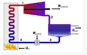
Fig : Ranking Cycle

1-2 : Iscentropic Expansion in the Turbine (Where the steam from the boiler is converted into meachanical energy).

2-3 : Constant Pressure Heat Rejection in the Condensor (Pressure heat rejection take place where the vapour is converted to liquid inside a condensor).

3-4 : Iscentropic Expansion in the Pump (In the pump where the pressure increases and the liquid is fed to the boiler).

4-1 : Constant Pressure Heat Addition in Boiler (inside the boiler from where the superheated steam is fed the Turbine)

Thermodynamic Equations and Formula :

for Iscentropic Expasion

`(T2)/(T1)=((P2)/(P1))^(1-(1/gamma))`

Where,

T is the Temperature at that state (K),

P is Pressure at the state (bar),

gamma is heat capacity ratio.

for neat work(W_net) abd back work ratio(Bw_rato) :

W_net = Wt-Wp

Bw(ratio) = Wp/Wt

Wt = h1-h2

Wp = h4-h3

where,

h is enthalpy at that state (kJ/kg),

W_t is Turbine work (kJ/kg),

W_p is Pump work (kJ/kg).

For Thermal Efficiency (ηt) :

ηt = W_net/(Q_in)

Q_in = h1-h4

Where,

Q_in is Heat added by the bolier (J);

h is Enthalpy atthat state (kJ/kg)

Explanation of code :

• The give inputs are entered.
• Using the XSteam table and the thermodynamic equation the various state varibles such as Pressurs, Temperature, Enthalpy and entropy are calculated.
• The net work done (W_net), Back work ratio and thermal efficiency of the system are calculated.
• Graphs are plotted to get the T-S and H-S diagram of the ranking cycle.

code :

clear all
close all 
clc

disp('RANKING CYCLE');
disp('1-2 is Iscentropic Expansion in the Turbine');
disp('2-3 is Constant Pressure Heat rejection by the Condesor');
disp('3-4 is Iscentropic Expansion in the Pump');
disp('4-1 is Constant Pressure Heat addition to the Boiler');

% Input
disp('INPUTS');
P1 = input('Enter the Pressure at turbine inlet(bar):');
T1 = input('Enter the Temperature at the Turbine inlet(degree C):');
P2 = input('Enter the Pressure at the Condensor(bar):');

% using the XSteam function, the enthalpy and entropy at various
% Points can be calculated

% Calculating enthalpy(h) and entropy(s) at point 1:
h1 = XSteam('h_pT',P1,T1);

s1 = XSteam('s_pT',P1,T1);

% Caluclating pressure(p), enthalpy(h) and entropy(s) at point 2

% Since Iscentropic Expansion

s2=s1

% For Iscentropic Expansion 

% wkt (T2/T1) = (P2/P1)^(1-(1/g))
g = 1.4;
power = 1-(1/g);

% Hence (T2/T1) = (P2/P1)^power 
T2 = T1*((P2/P1)^power);
h2 = XSteam('h_pT',P2,T2);

% Caluclating pressure(p), enthalpy(h) and entropy(s) at point 3

% Since Constant Pressure Heat Removal
P3 = P2;
T3 = T2;
h3 = XSteam('hL_T',T3);
s3 = XSteam('sL_T',T3);

% Caluclating pressure(p), enthalpy(h) and entropy(s) at point 4

% Since Iscentropic Compression
s4 = s3;

% Since Constant Pressure Process
P4 = P1;

T4 = XSteam('T_ps',P4,s4);
h4 = XSteam('h_pT',P4,T4);
h41 = XSteam('hL_p',P4);
s41 = XSteam('sL_p',P4);
h42 = XSteam('hV_p',P4);
s42 = XSteam('sV_p',P4);
T41 = XSteam('T_hs',h41,s41);
T42 = XSteam('T_hs',h42,s42);

% Calculating the Entropy and Enthapy at the saturation curve

Temp = linspace(0,500,600);

for i = 1:length(Temp)
sv(i) = XSteam('sV_T',Temp(i));
sl(i) = XSteam('sL_T',Temp(i));

hv(i) = XSteam('hV_T', Temp(i));
hl(i) = XSteam('hL_T', Temp(i));

end

% Calculating Net Work output(W_pnet)

W_t = h1-h2;
W_p = h4-h3;
W_net = W_t-W_p;

% Calculating Back Work Raio
Bw_ratio = W_p/W_t;

% calculating the Thermal efficiency
Q_in = h1-h4;
eff_thermal = (W_net/Q_in)*100;

% Calculating Specific Steam cosumption
% wkt 1j =3600kg/s
SSC = 3600/W_net;

% Displaying Results in the command window
disp('Resulats');
P1 = P1;
T1 = T1;
P2 = P2;
disp('At stage point 1');
n1 = sprintf('P1 is %.3f bar',P1);
disp(n1)
n2 = sprintf(T1 is %.3f C',T1)
disp(n2);
n3 = sprintf('h1 is %.3f kJ/kg',h1);
disp(n3);
n4 = sprintf('s1 is %.3f kJ/kgK',s1);
disp(n4);

disp('At stage point 2');
n11 = sprintf('P2 is %.3f bar',P2);
disp(n11);
n21 = sprintf('T2 is %.3f C',T2);
disp(n21);
n31 = sprintf('h2 is %.3f kJ/kg',h2);
disp(n31);
n41 = sprintf('s2 is %.3f kJ/kgK',s2);
disp(n41);

disp('At stage point 3');
n12 = sprintf('P2 is %.3f bar',P2);
disp(n12);
n22 = sprintf('T2 is %.3f C',T2);
disp(n22);
n32 = sprintf('h2 is %.3f kJ/kg',h2);
disp(n32);
n42 = sprintf('s2 is %.3f kJ/kgK',s2);
disp(n42);

disp('At stage point 4');
n13 = sprintf('P2 is %.3f bar',P2);
disp(n13);
n23 = sprintf('T2 is %.3f C',T2);
disp(n23);
n33 = sprintf('h2 is %.3f kJ/kg',h2);
disp(n33);
n43 = sprintf('s2 is %.3f kJ/kgK',s2);
disp(n43);

n14 = sprintf('W_t is %.3f kJ/kg',W_t);
disp(n14);
n15 = sprintf('W_p is %.3f kJ/kg',W_p);
disp(n15);
n16 = sprintf('W_net is %.3f kJ/kg',W_net);
disp(n16);
n17 = sprintf('eff_thermal is %.2f Percent',eff_thermal);
disp(n17);
n18 = sprintf('SSC is %.2f kg/kwh',SSC);
disp(n18);

figure(1)
plot([s1 s2],[T1 T2],[s2 s3],[T2 T3],[s3 s4],[T3 T4],[s4 s41],[T4 T41],[s41 s42],[T41 T42],[s42 s1],[T42 T1],'marker','*','color','r')
hold on
plot(sv,Temp)
plot(sl,Temp)
xlabel('Entropy-s(kJ/kgK');
ylabel('Temperature-T(K)');

figure(2)
plot([s1 s2],[h1 h2],[s2 s3],[h2 h3],[s3 s4],[h3 h4],[s4 s1],[h4 h1],'marker','*','color','g')
hold on
plot(sv,hv)
plot(sl,hl)
xlabel('Entropy-s(kJ/kgK');
ylabel('Enthalpy-h(kJ/k)');
 

Output :

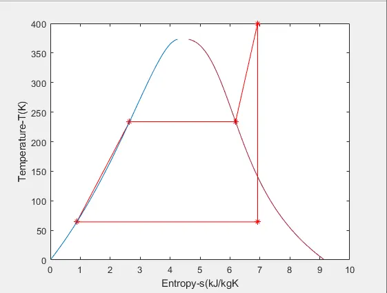
T-S diagram :

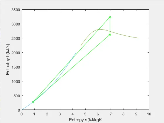
H-S diagram :

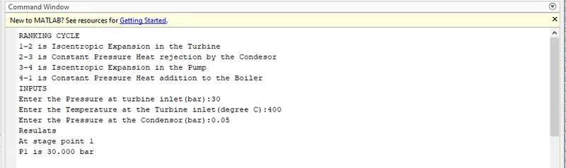
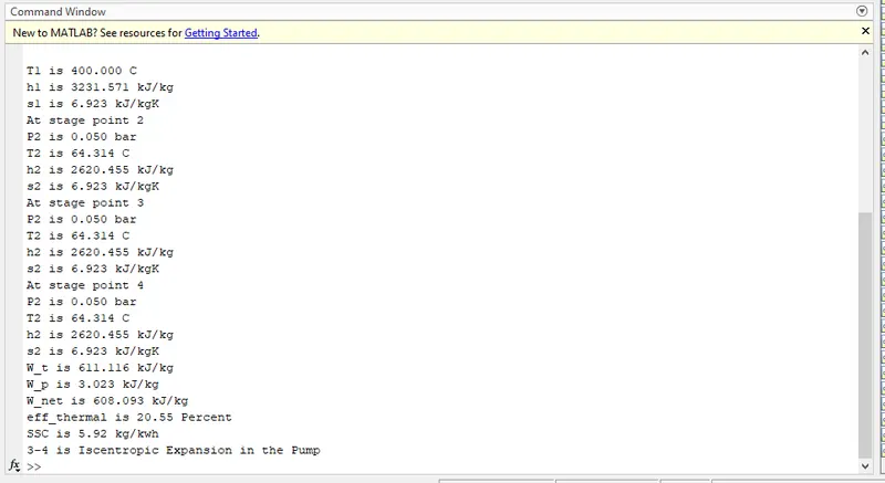
Command Window :

Results and conclusion :

• The performance of the Heat Engine was calculated and the following observation were made.

1. net Work = 608.093 kJ/kg
2. Thermal efficiency = 20.55%
3. Back Work Ratio = 0.4%

• The T-S and H-S performance curves of ranking cycle were plotted.