Week 3 - Solving second order ODEs
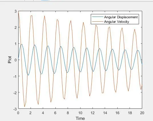
Aim: To write a matlab code to simulate the motion of a simple Pendulum ( ODE `(d^2theta)/dt^2 +b/m (d theta)/dt +g/lsin theta = 0` )between 0-20 sec, for angular displacement=0,angular velocity=3 rad/sec at time t=0.
Governing Equation:
`(d^2theta)/dt^2 +b/m (d theta)/dt +g/lsin theta = 0`
In the above equation,
g = gravity in m/s2,
l = length of the pendulum in m,
m = mass of the ball in kg,
b = damping coefficient.
Theory:
An ordinary differential equation (also abbreviated as ODE), in Mathematics, is an equation which consists of one or more functions of one independent variable along with their derivatives. A differential Equation is an equation that contains a function with one or more derivatives. But in the case ODE, the word ordinary is used for derivative of the functions for the single independent variable.
In case of other types of differential equations, it is possible to have derivatives for functions more than one variable. The types of DEs are Partial Differential Equation, linear and non-linear differential equations, homogeneous and non-homogeneous differential equation.
ODE45 function in MATLAB
Ode45 is a function in matlab that solves ordinary or partial differential equation using a numerical method. The numerical method in question here is the 4th order Runge Kutta method.
The function ode45 takes 3 inputs. The 3 inputs are the function to be integrated,the time span (integration limits) and initial condition.
The solver will choose a step size that is most suitable for the solution to obtain solution in the most optimal time possible.
The function can be provided in the form of an anonymous function,
[t,results] = ode45(@(x)x^2,tspan,y0)
Creating 2 first order ODE's
when `theta = theta1`
`(d theta)/dt = (d theta1)/dt = theta2`........1
`(d^2theta)/dt^2 = (d^2theta1)/dt^2 = (d theta2)/dt`..........2
now,
`(d^2theta)/dt^2 +b/m (d theta)/dt +g/lsin theta = 0`
substituting `theta = theta1`
`(d^2theta1)/dt^2 +b/m (d theta1)/dt +g/lsin theta1 = 0`
`(d theta2)/dt +b/m (theta2)+g/lsin theta1 =0`.......................from 1 & 2
Therefore,
`(d theta1)/dt = theta2`........1st ODE
`(d theta2)/dt = -b/m - g/l(sintheta1)`.......2nd ODE
In matrix form
`d/dt[theta1;theta2] = [theta2 ; -b/m -g/lsintheta1]`
Procedure
1) The function code is with reference to the above derived two 1st order ODE , where we create an array of `d/dt[theta1;theta2] = [theta2 ; -b/m -g/lsintheta1]` and use ode45 command to solver the ode.
2) The main code starts with clear all,close all,clc .
3) Appropriate inputs , initial condition, and integration limits is mentioned and the same is written in code.
4) Now, we call the function into the main program.
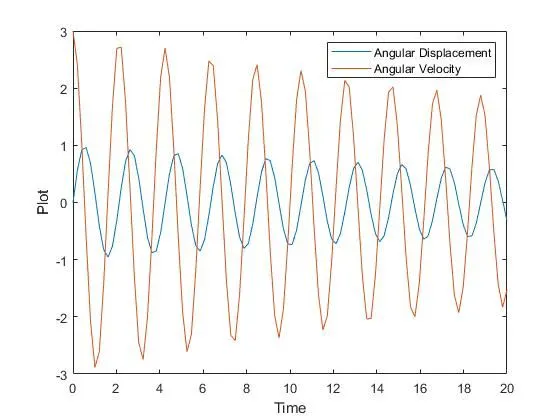
5) The results of the displacement and velocity is then plotted with the plot command we get a graph for the time span.
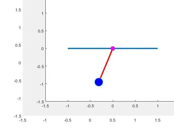
6) we use the for loop to plot the pendulum positions for the range of displacement and angular velocity values and each position is stored in different frames for creation of an animation.
7) An animation is then created by stiching each frames with help of movie, getframes,VideoWriter and write video commands.
Matlab function code:
function [dtheta_dt] = ode_func(t,theta,b,g,l,m)

theta1 = theta(1)
theta2 = theta(2)
dtheta1_dt = theta2;
dtheta2_dt = -(b/m)*theta2 - (g/l)*sin(theta1);
dtheta_dt = [dtheta1_dt; dtheta2_dt];
end
Matlab code:
clear all
close all
clc

%Inputs
b=0.05;
g=9.81;
l=1;
m=1;

% Initial condition
theta_0 = [0;3];

%time points
t_span = linspace(0,20,100);

%solve ODE
[t, results] = ode45(@(t,theta) ode_func(t,theta,b,g,l,m),t_span, theta_0);

figure(1)
plot(t,results(:,1))
hold on
plot(t,results(:,2))
ylabel('Plot')
xlabel('Time')
legend('Angular Displacement','Angular Velocity')

% looping
ct=1;

for i = 1:length(results(:,1))

 x0 = 0;
 y0 = 0;

 x1 = l*sin(results(i,1));
 y1 = -l*cos(results(i,1));

 figure(2)
 plot([-1 1],[0 0],'linewidth',3)
 hold on
 axis([-1.5 1.5 -1.5 1.5])
 plot([x0 x1],[y0 y1],x1,y1,'linewidth',4,'color','r')
 plot(x0,y0,'o','markersize',10,'markerfacecolor','m')
 plot(x1,y1,'marker','o','markersize',20,'markerfacecolor','b','markeredgecolor','c')
 pause(0.1)
 hold off
M(ct) =getframe(gcf);
ct = ct+1;
end

movie(M)
videofile = VideoWriter('Pendulum.avi','Uncompressed AVI');
videofile.FrameRate = 10
open(videofile)
writeVideo(videofile,M)
close(videofile)
output:
Displacement vs Velocity
Pendulum animation figure:
Error 1
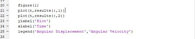
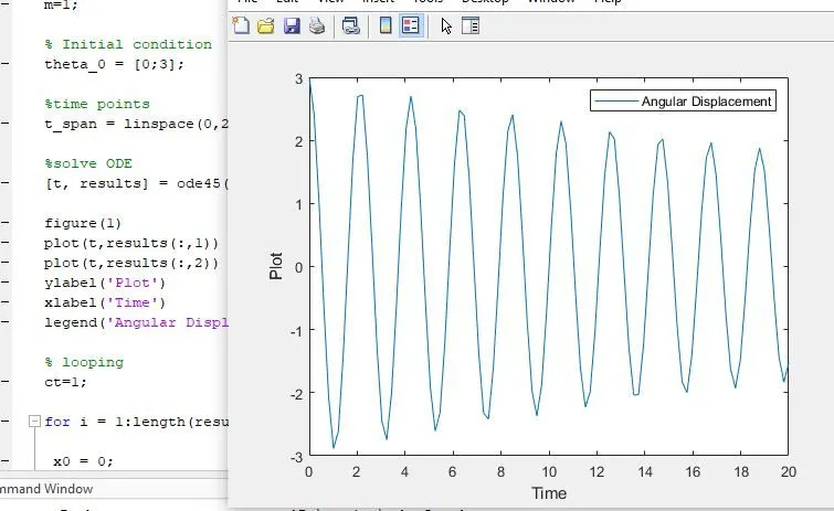
Solution_for_error 1: The displacement plot was not displaced in the same plot.
Used Hold on command to dispaly both the velocity and displacement in the same figure.
Error 2:
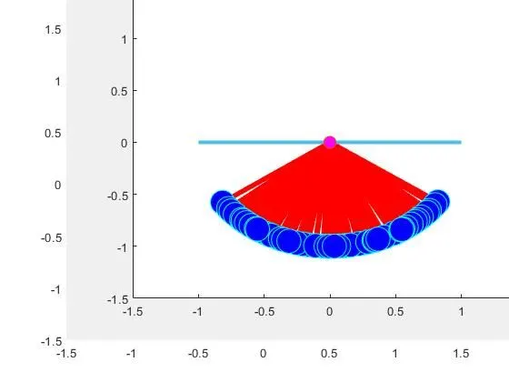
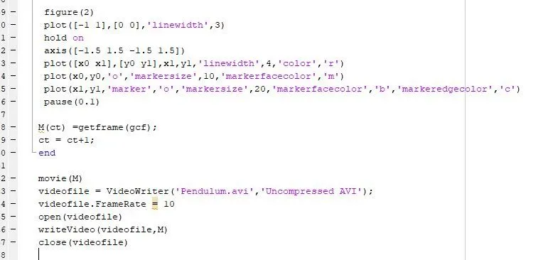
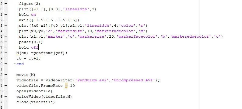
solution : All the frames captured are displaying in the samefigure due to this the animation file is displaying as shown above.
hold off command by used before storing the frames in M(ct)
Youtube_Video_link:
References: