Week 3 - Solving second order ODEs

ANSWER:

AIM: write a program that solves the following ODE. This ODE represents the equation of motion of a simple pendulum with damping

In the above equation,

g = gravity in m/s2,

L = length of the pendulum in m,

m = mass of the ball in kg,

b=damping coefficient.

use,

L=1 metre,

m=1 kg,

b=0.05.

g=9.81 m/s2.

WORKING OF SIMPLE PENDULUM

A simple pendulum consists of a metal bob hung by a string connected to a pivot point. The bob oscillates in to and fro motion because of its mass and momentum. The movement from mean to one extreme and then to the other extreme and again back to the mean is called a complete oscillation.

CODE FOR SIMPLE PENDULUM

close all
clear all
clc
 % Simulating program for pendulum 
% initial parameters
b = 0.05;
g = 9.81;
l = 1;
m = 1;

%Initial condition
theta_0 = [0;3];

% time points 
t_span = linspace(0,20,500);

% solve ODE Equation of first order
[t,results] = ode45(@(t,theta) ode_func(theta,b,g,l,m),t_span,theta_0);

%Plotting on graph
plot(t,results(:,l))
hold on
plot(t,results(:,2))
xlabel('Time')
ylabel('angular displacement and angular velocity')
title('Pendulum displacement') 
legend('angular displacement','Angular velocity')
hold off
grid on
% Animation of pendulum

ct = 1;

for i = 1:length(t)
    
    x = sin(results(i,1))*l;
    y = -cos(results(i,1))*l;
    
    figure(2)
    
    plot([-1,1],[0,0],'linewidth',15)
    hold on
    plot([0,x],[0,y],'linewidth',10)
    plot(x,y,'Marker','o','Markersize',20,'Markerfacecolor','g')
    hold off
    axis([-1.5,1.5,-2,2]);
    xlabel('x axis')
    ylabel('y axis')
    title('Pendulum oscillation')
   
   M(ct) = getframe(gcf);
    ct = ct+1;
end

% creating movie of pendulum movement

movie(M);
videofile = VideoWriter('pendulum_animation.avi','Uncompressed AVI');
open(videofile);
writeVideo(videofile,M);
close(videofile);

   % END OF THE CODE

CODE TO RUN FUNCTION

function[dtheta_dt] = ode_func(theta,b,g,l,m)

theta1 = theta(1);
theta2 = theta(2);

dtheta1_dt = theta2;

dtheta2_dt = -(b/m)*theta2-(g/l)*sin(theta1);


[dtheta_dt] = [dtheta1_dt;dtheta2_dt];
end

EXPLANATION OF CODE:

• START THE CODE FROM
• Clear all
• close all
• clc
• defining the input parameters (damping coefficient, length,gravity of earth,mass of thye ball) & initial conditions as (angular displacement , angular velocity)
• then time is ngiven from 0 to 20 secomds for 500 frames ( i.e, the time is equispaced between 0 & 10 values)
• then the ode function is used to solve the derivation of simple pendulum
• the ode function is called along with the time and the theta
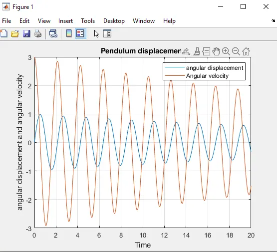
• then the graph is plotted for the angular velocity ,angular displacement vs time
• to show the simulation of a simple pendulum for loop is created
• to create the movie , we used the videowriter
• the animation is opened ,written and closed to provide an animation contineously.

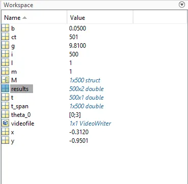
WORKSPACE

COMMAND WINDOW

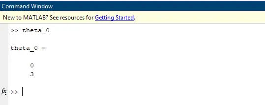
the output is shown below

PLOT AND ANIMATION LINK:

The plot is generated between the angular displacement , angular velocity vs time the animation is generated foer the simple pendulunm in required format

AMIMATION LINK:

https://youtu.be/Ojzp_PEFaFk