Project 2 - Rankine cycle Simulator
ANSWER:
RANKINE CYCLE:
The Rankine cycle is an idealized thermodynamic cycle describing the process by which certain heat engines, such as steam turbines or reciprocating steam engines, allow mechanical work to be extracted from a fluid as it moves between a heat source and heat sink. The Rankine cycle is named after William John Macquorn Rankine, a Scottish polymath professor at Glasgow University.
Heat energy is supplied to the system via a boiler where the working fluid (typically water) is converted to a high pressure gaseous state (steam) in order to turn a turbine. After passing over the turbine the fluid is allowed to condense back into a liquid state as waste heat energy is rejected before being returned to boiler, completing the cycle. Friction losses throughout the system are often neglected for the purpose of simplifying calculations as such losses are usually much less significant than thermodynamic losses, especially in larger systems.
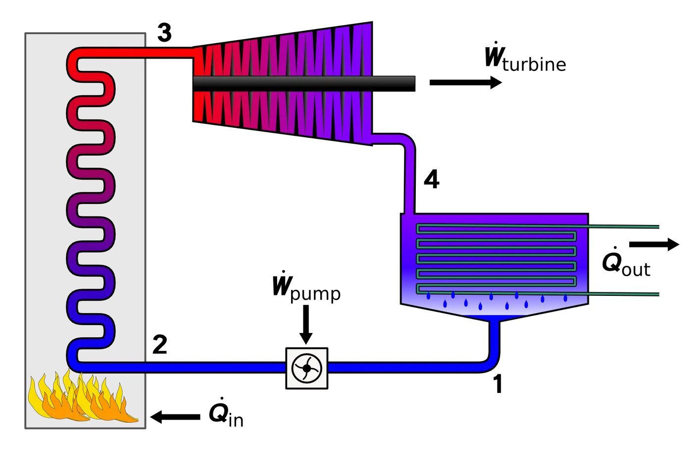
COMPONENTS OF RANKINE CYCLE:
- Pump: Compression of the fluid to high pressure using a pump (this takes work)
- Boiler: The compressed fluid is heated to the final temperature (which is at boiling point), therefore, a phase change occurs—from liquid to vapor.
- Turbine: Expansion of the vapor in the turbine.
- Condenser: Condensation of the vapor in the condenser (where the Waste heat goes to the final heat sink (the atmosphere or a large body of water
DESCRIPTIOIN:
The Rankine cycle closely describes the process by which steam engines commonly found in thermal power generation plants harness the thermal energy of a fuel or other heat source to generate electricity. Possible heat sources include combustion of fossil fuels such as coal, natural gas, or oil, renewable fuels like biomass or ethanol, nuclear fission, and concentrated solar power. Common heat sinks include ambient air above or around a facility and bodies of water such as rivers, ponds, and oceans.
The ability of a Rankine engine to harness energy depends on the relative temperature difference between the heat source and heat sink. The greater the differential, the more mechanical power can be efficiently extracted out of heat energy, as per Carnot's theorem.
The efficiency of the Rankine cycle is limited by the high heat of vaporization of the working fluid. Unless the pressure and temperature reach super critical levels in the boiler, the temperature range that the cycle can operate over is quite small: Steam turbine entry temperatures are typically around 565 °C and condenser temperatures are around 30 °C. This gives a theoretical maximum Carnot efficiency for the turbine alone of about 63.8% compared with an actual overall thermal efficiency of less than 50% for typical power stations. This low steam turbine entry temperature (compared to a gas turbine) is why the Rankine (steam) cycle is often used as a bottoming cycle to recover otherwise rejected heat in combined-cycle gas turbine power stations.
Rankine engines generally operate in a closed loop where the working fluid is reused. The water vapor with condensed droplets often seen billowing from power stations is created by the cooling systems (not directly from the closed-loop Rankine power cycle). This 'exhaust' heat is represented by the "Qout" flowing out of the lower side of the cycle shown in the T–s diagram below. Cooling towers operate as large heat exchangers by absorbing the latent heat of vaporization of the working fluid and simultaneously evaporating cooling water to the atmosphere.
While many substances can be used as the working fluid, water is usually chosen for its simple chemistry, relative abundance, low cost, and thermodynamic properties. By condensing the working steam vapor to a liquid the pressure at the turbine outlet is lowered and the energy required by the feed pump consumes only 1% to 3% of the turbine output power and these factors contribute to a higher efficiency for the cycle. The benefit of this is offset by the low temperatures of steam admitted to the turbine(s). Gas turbines, for instance, have turbine entry temperatures approaching 1500 °C. However, the thermal efficiency of actual large steam power stations and large modern gas turbine stations are similar.
The four processes in the Rankine cycle:
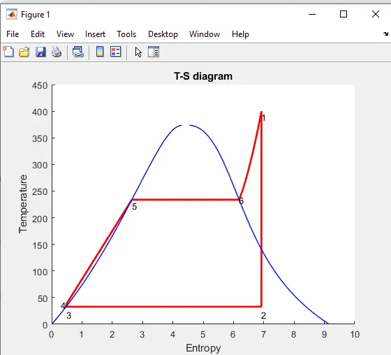
There are four processes in the Rankine cycle. The states are identified by numbers (in brown) in the T–s diagram
process 1-2 : Isentropic expansion in the turbine :- In the turbine, the high pressure and temperature steam is expanded isentropically over the turbine blades. The turbine work output is obtained Wt.
process 2-3 : Isobaric heat rejection in condenser :- In condenser, the exhaust gases from the turbine are cooled using external water. The hot steam is condensed into water and then fed to the pump. The heat rejected from the water Qout.
process 3-4 : Isentropic compression in pump :- The condensate from the condenser is again fed into the boiler tube with increased pressure. Work done by the pump Wp.
process 4-1 : Isobaric heat addition in boiler :- The heat is added to the water by firing of coal inside it. Due to addition of heat, the water is gets converted into the steam. Heat added to the water in the boiler, Qin.
EQUATIONS:
In general, the efficiency of a simple rankine cycle can be written as

Each of the next four equations is derived from the energy mass balance for a control volume.  defines the thermodynamic efficiency of the cycle as the ratio of net power output to heat input. As the work required by the pump is often around 1% of the turbine work output, it can be simplified.




When dealing with the efficiencies of the turbines and pumps, an adjustment to the work terms must be made:


We have to find:
1. net work output (KJ/Kg)
2. Back work ratio
CODE FOR RANKINE CYCLE SIMULATOR:
%  RANKINE CYCLE SIMULATOR  %
clear all
close all
clc
%  rankine cycle processes %
fprintf(' RANKINE CYCLE SIMULATOR')
fprintf('\n1-2 Isentropic expansion in Turbine')
fprintf('\n2-3 Isobaric heat rejection by condensor')
fprintf('\n3-4 Isentropic compression in pump')
fprintf('\n4-1 Isobaric heat addition by boiler \n')
fprintf('\n')
% Given inputs %
P1 = input('pressure at turbine inlet (bar) :');
T1 = input('temperature at turbine inlet (celsius) :');
P2 = input('pressure at condensor (bar) :');

%  Stage -1 (Turbine inlet)  %
% pressure and temperatures are given %
h1 = XSteam('h_pT',P1,T1);
s1 = XSteam('s_pT',P1,T1);

%  Stage - 2 (Condenser inlet)  %
% P2 is given % to find h2 %
% h2 = hf2 + x2 (hg2 - hf2) %
% Where x2 = (s2 - sf2)/(sg2 - sf2) %
s2 = s1 ; % Isentropic process
sf2 = XSteam('sL_p',P2);
sg2 = XSteam('sV_p',P2);
x2 = (s2-sf2)/(sg2-sf2);
hf2 = XSteam('hL_p',P2);
hg2 = XSteam('hV_p',P2);
h2 = hf2 + (x2*(hg2 - hf2));

%  Stage - 3 (Pump inlet)  %
P3 = P2; % Isobaric process
% saturated liquid stage %
h3 = XSteam('hL_p',P3);
s3 = XSteam('sL_p',P3);
T3 = XSteam('Tsat_p',P3);
T2 = T3; % for stage - 2

% Stage - 4 (Boiler inlet) %
s4 = s3; % Isentropic process
P4 = P1; % Isobaric process
h4 = XSteam('h_ps',P4,s4);
% to find T4 % T3/T4 = (P3/P4)^((C-1)/C) %
% Where C = Cp4/Cv4
% Specific heat values %
Cp4 = XSteam('Cp_ps',P4,s4); % constant pressure %
Cv4 = XSteam('Cv_ps',P4,s4); % constant volume %
C = Cp4/Cv4;
T4 = T3/((P3/P4)^((C-1)/C));
% saturated liquid state %
T5 = XSteam('Tsat_p',P1);
s5 = XSteam('sL_p',P1);
h5 = XSteam('hL_p',P1);
% saturated vapour state %
T6 = T5;
s6 = XSteam('sV_p',P1);
h6 = XSteam('hV_p',P1);
% Calculation of work (KJ/Kg) %
Wt = h1 - h2; % Turbine work
Wp = h4 - h3; % Pump work
W = Wt - Wp; % Net work Output
% Calculation of heats %
Qin = h1 - h4; % heat addition in boiler
Qout = h2 - h3; % heat removed in condeser
% Thermal Efficiency (%) %
nTherm = (W/Qin)*100;
% Steam rate (Kg/KWh) %
SSC =3600/W;
% Back work ratio %
BWR = Wp/Wt;


% ============================== Plotting =============================== %
% plotting T-S diagram %
figure(1)
hold on
title('T-S diagram')
plot([s1 s2],[T1 T2],'linewidth',2,'color','r')
plot([s2 s3],[T2 T3],'linewidth',2,'color','r')
plot([s3 s4],[T3 T4],'linewidth',2,'color','r')
plot([s4 s5],[T4 T5],'linewidth',2,'color','r')
plot([s5 s6],[T5 T6],'linewidth',2,'color','r')
s_1 = linspace(s6,s1,500);
for j = 1:length(s_1);
 t_1(j) = XSteam('T_ps',P1,s_1(j));
end
plot(s_1,t_1,'linewidth',2,'color','r')
xlabel('Entropy')
ylabel('Temperature')
% plot saturation curve %
T = linspace(1,T1,500);
for i = 1:length(T);
 h_l(i) = XSteam('hL_T',T(i));
 h_v(i) = XSteam('hV_T',T(i));
 s_l(i) = XSteam('sL_T',T(i));
 s_v(i) = XSteam('sV_T',T(i));
end
plot(s_l,T,'linewidth',1,'color','b')
plot(s_v,T,'linewidth',1,'color','b')
% annotations %
text(s1,T1,'1','verticalalignment','top')
text(s2,T2,'2','verticalalignment','cap')
text(s3,T3,'3','verticalalignment','cap')
text(s4,T4,'4','horizontalalignment','right')
text(s5,T5,'5','verticalalignment','top')
text(s6,T6,'6','horizontalalignment','left')
% plotting H-S diagram %
figure(2)
hold on
title('H-S diagram')
plot([s1 s2],[h1 h2],'linewidth',2,'color','r')
plot([s2 s3],[h2 h3],'linewidth',2,'color','r')
plot([s3 s4],[h3 h4],'linewidth',2,'color','r')
h_4 = linspace(h4,h5,500);
for k = 1:length(h_4)
 s_4(k) = XSteam('s_ph',P1,h_4(k));
end
h_6 = linspace(h6,h1,500);
for m = 1:length(h_6)
 s_6(m) = XSteam('s_ph',P1,h_6(m));
end
plot(s_4,h_4,'linewidth',2,'color','r')
plot([s5 s6],[h5 h6],'linewidth',2,'color','r')
plot(s_6,h_6,'linewidth',2,'color','r')
xlabel('Entropy')
ylabel('Enthalpy')
% plot saturation curve %
plot(s_l,h_l,'linewidth',1,'color','b')
plot(s_v,h_v,'linewidth',1,'color','b')
% annotations %
text(s1,h1,'1','verticalalignment','top')
text(s2,h2,'2','verticalalignment','cap')
text(s3,h3,'3','verticalalignment','top')
text(s4,h4,'4','horizontalalignment','right')
text(s5,h5,'5','verticalalignment','top')
text(s6,h6,'6','verticalalignment','bottom')
% Results window %
fprintf('\n RESULTS')
fprintf('\n >>>At state point 1 :')
fprintf('\n P1 is : %f Bar',P1)
fprintf('\n T1 is : %f Deg celcius',T1)
fprintf('\n H1 is : %f KJ/Kg',h1)
fprintf('\n S1 is : %f KJ/KgK',s1)
fprintf('\n')
fprintf('\n >>>At state point 2 :')
fprintf('\n P2 is : %f Bar',P2)
fprintf('\n T2 is : %f Deg celcius',T2)
fprintf('\n H2 is : %f KJ/Kg',h2)
fprintf('\n S2 is : %f KJ/KgK',s2)
fprintf('\n')
fprintf('\n >>>At state point 3 :')
fprintf('\n P3 is : %f Bar',P3)
fprintf('\n T3 is : %f Deg celcius',T3)
fprintf('\n H3 is : %f KJ/Kg',h3)
fprintf('\n S3 is : %f KJ/KgK',s3)
fprintf('\n')
fprintf('\n >>>At state point 4 :')
fprintf('\n P4 is : %f Bar',P4)
fprintf('\n T4 is : %f Deg celcius',T4)
fprintf('\n H4 is : %f KJ/Kg',h4)
fprintf('\n S4 is : %f KJ/KgK',s4)
fprintf('\n')
fprintf('\n Turbine work : %f KJ/Kg',Wt)
fprintf('\n Pump work : %f KJ/Kg',Wp)
fprintf('\n Net work output : %f KJ/Kg',W)
fprintf('\n Thermal efficiency : %f percent',nTherm)
fprintf('\n SSC : %f Kg/KWh',SSC)
fprintf('\n Back work ratio : %f',BWR)
fprintf('\n')
Code explanation :
• The program is started with the clear all close all clc commands .
• Information about the cycle and their processes are mentioned using the 'fprintf' command.
• Input variables P1, T1 and P2 are given by 'input' command whose values are to be entered in command window while executing .
• The properties values of steam and water are extracted from the XSteam.m file.
• At state 1, the values for the enthalpy and entropy are extracted as a function of temperature and pressure.
• Similarly, at all states are extracted.
• Formula for calculating the unknown state values of temperature, pressure, enthalpy and entropy are calculated from the basic formulas from reference book.
• After calculating the values at all states, work done and heat transfer are calculated.
• The efficiency, specific steam consumption and back work ratio are also calculted using the above formulas.
• The saturation curve is plotted, temperature range is defined using the 'linspace' command and values of enthalpy and entropy are calculated at each temperature point. These values are used to draw the saturation curves in the h-s and t-s diagrams.
• Now the cycle is plotted over the saturation curve and annotations for each process are specified using the 'text' command.
• All the results of the Rankine cycle are plotted using the 'fprintf' command.
OUTPUT:
 RANKINE CYCLE SIMULATOR
1-2 Isentropic expansion in Turbine
2-3 Isobaric heat rejection by condensor
3-4 Isentropic compression in pump
4-1 Isobaric heat addition by boiler

pressure at turbine inlet (bar) :30
temperature at turbine inlet (celsius) :400
pressure at condensor (bar) :0.05

 RESULTS
 >>>At state point 1 :
 P1 is : 30.000000 Bar
 T1 is : 400.000000 Deg celcius
 H1 is : 3231.571027 KJ/Kg
 S1 is : 6.923259 KJ/KgK

 >>>At state point 2 :
 P2 is : 0.050000 Bar
 T2 is : 32.875490 Deg celcius
 H2 is : 2110.708212 KJ/Kg
 S2 is : 6.923259 KJ/KgK

 >>>At state point 3 :
 P3 is : 0.050000 Bar
 T3 is : 32.875490 Deg celcius
 H3 is : 137.765119 KJ/Kg
 S3 is : 0.476254 KJ/KgK

 >>>At state point 4 :
 P4 is : 30.000000 Bar
 T4 is : 36.935287 Deg celcius
 H4 is : 140.762226 KJ/Kg
 S4 is : 0.476254 KJ/KgK

 Turbine work : 1120.862815 KJ/Kg
 Pump work : 2.997107 KJ/Kg
 Net work output : 1117.865709 KJ/Kg
 Thermal efficiency : 36.167417 percent
 SSC : 3.220423 Kg/KWh
 Back work ratio : 0.002674
>>
PLOT FOR T-S :
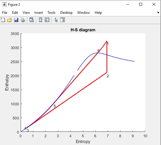
PLOT FOR H-S;
CONCLUSION:
The values of the net work output and the back work ratio are obtained by using the T-S and the H-S diagram and the state points are calculated.
REFERENCE: