Week 3 - Solving second order ODEs

In Engineering, ODE is used to describe the transient behavior of a system. A simple example is a pendulum

The way the pendulum moves depends on the Newtons second law. When this law is written down, we get a second order Ordinary Differential Equation that

describes the position of the "ball” w.r.t time.

Similarly, there are hundreds of ODESs that describe key phenomena and if you have the ability to solve these equations then you will be able to simulate any of

these systems.

Program code:

% a program to find the oscillation of an simple pendulum by using ODE45
% this is the main program
% clear all
close all
clc
%input data

b=0.2; %damping coefficient
m= 1; % mass of the bob in kg
l = 1; % length of the pendulum in meter
g = 9.81; %accleration due to gravity

%initial conditions
theta_0 = [0;5];

%time period of 20 seconds
t_span= linspace(0,50,500);
[t, result]= ode45(@(t,theta) ode_challenge(t,theta,b,g,m,l),t_span,theta_0);
figure(1)
hold on
plot(t, result(:,1))
plot(t, result(:,2))
title('Damped Harmonic motion of a Simple Pendulum')
legend('Angular displacement’, ‘Angular velocity')
ylabel('Plot')
xlabel (" Time(seconds)")
hold on

T=2*(pi)*((l/g)^0.5)

ct=1;

for i=1:length(t)
    
    x0=0;
    y0=0;
    
    x1=l*sin(result(i,1));
    y1=-1*cos(result(i,1));
    
    figure(2)
    plot([x0 x1],[ y0 y1],'color','b','linewidth',1.5)
    hold on
    plot(x1,y1,'o','MarkerSize',20,'markerFacecolor','y')
    plot(x0,y0+0.09,'v','color','r','MarkerSize',20,'markerFacecolor','k')
    hold on
    plot(x1,y1,'-')
    hold off
    axis([-1.5 1.5 -2 1])
    pause (0.01)
    grid on
    
    M(ct)=getframe(gcf);
    ct=ct+1;
            
end

movie(M);
videofile=VideoWriter('Simple Pendulum.avi','Uncompressed AVI');
open(videofile);
writeVideo(videofile,M);
close(videofile);

Function code:

function[dt_t] = ode_challenge(t,theta,b,g,m,l)
theta1=theta(1);
theta2=theta(2);
dtheta1_dt=theta2;
dtheta2_dt= -((b/m)*theta2+(g/l)*sin(theta1));
dt_t = [dtheta1_dt;dtheta2_dt]

end

Methodology:

To track a simple pendulum osciallation through MATLAB, we can achive this by creating a function program of the formula which derives the output.

1.Required datas should be delclared in main program.i.e mass, damping coefficient, length, accleration due to gravity.

2. Assigning the initial conditions 'theta 0'.Initial displacement is zero and initial velocity is 5m/s.

3. Assign time span through linspace command.

4. ode45 function to get result. In-order to execute ode45 we need a function where it contains the required data,which can be integrated with time. When we run the function we get the graph of simple harmonic motion.

5. To get an video output, we need to do a loop for each and every angle and trace it down to get a video, by recording it as an video by 'Movie' command.

Errors face:

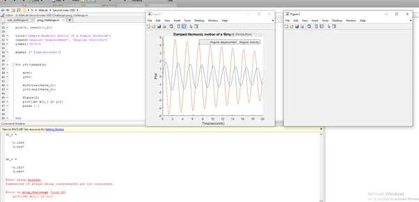
Typing errors

and invalid expression face frequently.

Result Video:

https://youtu.be/ddjSaBkPVbI