Week 3 - Solving second order ODEs

Link of Animation for Simple Pendulum as per given parameters:

https://youtu.be/yRgDA_pCSfg

The equation for the ODE for simple pendulum is given, so calculatting this equation.

here in the equation for theta = theta1 taken.

so equation getting

dtheta/dt = dtheta1/dt = theta2

so putting this values in the equation:

the final equation becomes to

dtheta2/dt = -[(b/m)*theta2]-[(g/l)*sin(theta1)]

using this equation creating a fuction. and this fuction called "ode_func"

code for the this "ode_func" is given below.

Below function code used as formula:

function [dtheta_dt] = ode_func(t,theta,b,g,l,m)

theta1 = theta(1)
theta2 = theta(2)
dtheta1_dt = theta2;
dtheta2_dt = -(b/m)*theta2-(g/l)*sin(theta1);
dtheta_dt = [dtheta1_dt;dtheta2_dt];

end

The code for calculating the ODE for equation of the motion of simple pendulum of the parameter given in the quation:

clear all
close all
clc

%Inputs:Damping coeffiecient(b),Accelaration of gravity(g)in m/s^2
%Inputs:Length of Pendulam(l)in m,Mass of Pendulam(m)in kg

b = 0.05;
g = 9.81;
l = 1;
m = 1;

%Initial condition

theta_0 = [0;3];

%Time points

t_span = linspace(0,20,500);

%Solve ODE

[t,results] = ode45(@(t,theta)ode_func(t,theta,b,g,l,m),t_span,theta_0);



%Combine result plot Red line for Displacement and green line for Velocity
figure(1)
plot(t,results(:,1),'Color','r')
hold on
plot(t,results(:,2),'Color','g')

ylabel(['Displacement(red color),Velocity-rad/sec(green color))'])
xlabel('Time-sec')

figure(2)
plot(results(:,1),results(:,2))
xlabel('Position(rad)')
ylabel('Angular Velocity(rad/Sec)')


theta2 = results(:,1);
ct = 1;
for i = 1:length(theta2);
    theta3 = theta2(i);

    x0 = 0;
    y0 = 0;
    x1 = l*sin(theta3);
    y1 = -l*cos(theta3);

    plot([-1.1 1.1],[0 0],'LineWidth',2);
    hold on
    plot([x0 x1],[y0 y1],'color','b','LineWidth',2)
    hold on
    plot(x1,y1,'o','Marker','o','markerfacecolor','magenta')
    hold off

    grid on

    axis([-1.5 1.5 -1.5 0.5])
    pause(0.005)
    M(ct) = getframe(gcf);
    ct = ct+1;
end
movie(M)
videofile = VideoWriter('simple pendulum.avi','Uncompressed AVI')
open(videofile)
writeVideo(videofile,M)
close(videofile)

The Result image is attached below:

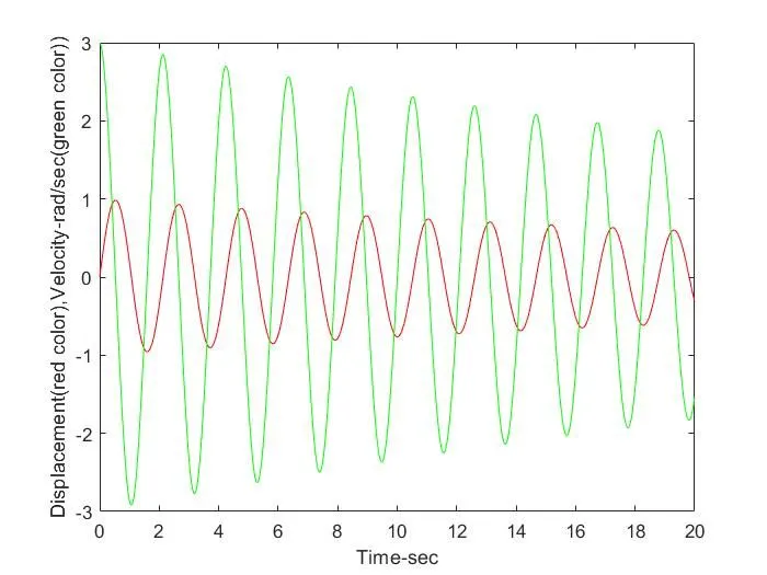
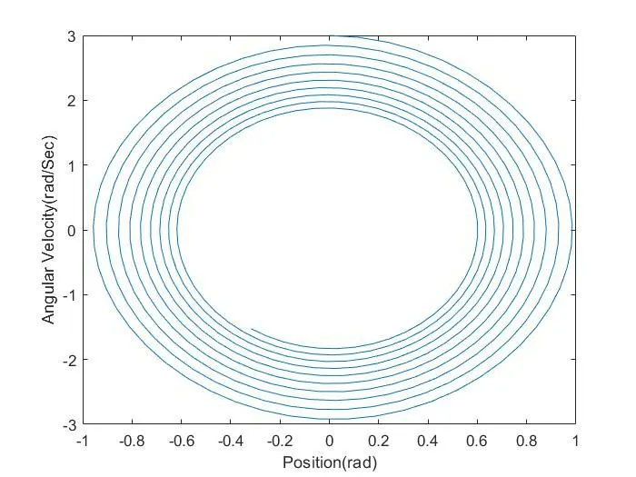
now creating a matlab code for making the animation for the movement of the simple pendulum.

so first of all defining all inputs which is used in the code:

b = damping coeeficient = 0.05

g = gravity Force in m/s = 9.81

l = lenth of the pendulum in m = 1

m = mass of the ball in kg = 1

now for dispacement start with 0 and velocity start with 3m/s at initial condition. so defining that as theta0 = [0,3]

now as given in the question simulation between 0-20s

so using linspace code defining 500values between 0 to 20s

now solving ODE

in matlab ODE45 command is inbuilt for solving ODE.

so using this command we use the fuction which is created "ode_func" and given time span and intial condition in the fuction.

in the output of this equation get the 2 coloum matrix in which first coloum is shows the values for the dispalcement with respect to time which is start from the 0.

and in the second coloum shows the values for the velocity with respect to time and its start from the 3.

now plotting this both so we can see clearly.

using plot command plotting this result and at xaxis shows the time in sec and at y axis shows two curves start in which the curve start with the 0 is of displacement and second curve which is start with 3 is of velocity in rad/sec.

and when plotting this both result in figure 2 we get the parabollic curve .

using for command creating the loop for the different position of the pendulum at different time so we can see the simulation of the simple pendulum.

now first of all we have to definie the position of the both end of the pendulum.

so we know that the pendulum is fixed at one end and move from the second end.

so at initial position we have define the fixed point at x0,y0

and for the other end we know that the

x1=l*sin(theta3) and y1=-l*cos(theta3)

because the point is in 4rd quaderent.

also for ball of pendulum use the marker command for the making the spear.

creating a loop for the diiferent position of the second point with respect to velocity and dispacement and plotting that using plot command.

now for animation video creating we use the movie command.

as a result see that the motion of the pendulum in the animation.

i have found some errors during this code run is :

getting some typing errors like upper case and lower case and some error of missing comma or bracket.

one erorr foundd during using the marker command . i have write the value 10 in marker command and error shows that marker command does not use the values. and so i have see that marker command is used for some special character some like 'o','*',etc. so i have put the 'o' for making spehere.

also i can't get animation at the end of result because i have write the values of x1 and y1 positive. but after that i have found that that is in fourth quaderent. so after correcting the equation i have run the simulation.