Week 3 - Solving second order ODEs

Aim: write a program that solves the following ODE. This ODE represents the equation of motion of a simple pendulum with damping

Theory:

In mathematics, a differential equation is an equation that relates one or more functions and their derivatives. In applications, the functions generally represent physical quantities, the derivatives represent their rates of change, and the differential equation defines a relationship between the two. Such relations are common; therefore, differential equations play a prominent role in many disciplines including engineering, physics, economics, and biology.

Simple Pendulum:

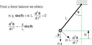
The simple pendulum consists of a point mass m hanging on a string of
length L from some support. One pulls the mass back
to some starting angle, θ 0, and releases it. The goal is to find the angular
position as a function of time.
There are a couple of possible derivations. We could either use Newton’s Second Law of Motion, F = ma, or its rotational analogue in terms of
torque, τ = Iα. We will use the former only to limit the amount of physics
background needed.
There are two forces acting on the point mass. The first is gravity. This
points downward and has a magnitude of mg, where g is the standard symbol for the acceleration due to gravity. The other force is the tension in the
string. these forces and their sum are shown. The magnitude
of the sum is easily found as F = mg sin θ.

The input parameters which is used in progaram are as follows

length of the string (l) = 1 meter

mass of the bob (m) = 0.1 kg

damping coefficients (b) = 0.05

accelaration due to gravity (g) = 9.81 m/s^s

initials condition of the pendulum

angular displacement = 0

angular velocity = 9 rad/sec

time = t

The second order differential eqaution:

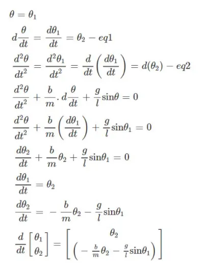
by solving for the value of theta1 and theta 2 we get the solution.

Methodology:

1. solving the second order differential equation
2. writing the code for solving the second order differential equation by using command ODE45 in MATLAB
3. defining and making a fuction for the value of theta1 and theta 2 for different parameters of the pendulum
4. plotting the motion for angular displacment and angular velocity w.r.t time.
5. followed by the animation of the simple pendulum

% code to solve second order differential equation
clear all
close all
clc

%damping coefficient 
b = 0.05;
%length of the string  in meter
l = 1;
% mass of the bob in kg
m = 0.1;
% accelaration due to gravity in m/s^2
g = 9.81;

%initial condition 
theta_0 = [0;5]; 
%time span
t_span = linspace(0,20,500);

%solving ode
[t, result] = ode45(@(t,theta)ode_function(t,theta,b,g,l,m),t_span,theta_0);

%plotting
plot (t, result(:,1))
hold on 
plot (t, result(:,2))
title ('damped harmonic motion of a pendulum')
legend ('angular displacement','angular velocity')
 xlabel 'time'
 ylabel 'plot'

 %for loop 
 
 %counter value
  ct =1;
  
for i = 1:length (result(:,1))
    x_start = 0;
    y_start = 0;
    x_end = 1*sin(result(i,1));
    y_end = -1*cos(result(i,1));
    
    %plotting the animation
    figure(2)
    plot ([-1 1],[0 0], 'linewidth',5)
    hold on
    plot([x_start x_end],[y_start y_end],'linewidth',3)
    
    plot (x_end,y_end,'o','markersize',30, 'markerfacecolor' ,'g')
    title (' animation of the pendulum')
    axis ([-1.5 1.5 -1.5 1.5])
    pause (0.03)
    hold off 
    M(ct) = getframe (gcf)
    ct = ct+1
end

%animation of the pendulum
 movie(M)
 videofile = VideoWriter('pendulumanimation.avi','uncompressed avi')
 write(videofile,M)
 close(videofile)

Conclusion:

Ordinary differential equations applications in real life are used to solve different problems like the motion of a simple pendulum,explain thermodynamic concept etc. the motion of the simple pendulum depend on the length of the string, mass of the bob and the damping coefficients. by changing the single parameters may change the angular displacment and the angular velocity w.r.t time

Results:

x_end = 0.2443

x_start = 0

y_end = -0.9697

y_start =0

function  [dtheta_dt] = ode_function(t,theta,b,g,l,m)

theta1 = theta(1) 
theta2 = theta(2)
dtheta1_dt = theta2;
dtheta2_dt = -(b/m)*theta2-(g/l)*sin(theta1);
dtheta_dt = [dtheta1_dt;dtheta2_dt];
end

Point to be noted :

the shared screenshots of plot are taken at different masses of the bob

the one screen shot shows at the mass 1kg

and the other one shows the plotting at maas 0.1kg