Week 3 - Solving second order ODEs

AIM: 1). To write the MATLAB program that solves ordinary diferential equation of motion of a simple pendulum with damping.

`(d^2 theta)/dt^2+(b/m)(d theta)/dt+(g/l)sintheta=0`

2). To write the MATLAB program that stimulates the pendulum motions.

THEORY: The motion of the pendulum depends upon the Newton's Second Law of motion. With this law we can get a second order differential equation that describes the motion of ball w.r.t. time.

`(d^2 theta)/dt^2+(b/m)(d theta)/dt+(g/l)sintheta=0`

in the above equation b= damping coefficient,

m = mass of the ball (kg),

g = gravity (m/s),

l = length of the pendulum(m).

Solving `2^(nd)`order ODE by converting into FIRST ORDER ODE.

while solving higher order ODE equations in matlab, first we have to convert them into series of first order differential equations.

here the equation `(d^2 theta)/dt^2+(b/m)(d theta)/dt+(g/l)sintheta=0` is in `2^(nd)` order.

`(d^2 theta)/dt^2+(b/m)(d theta)/dt+(g/l)sintheta=0`

let assume `theta = theta_1 ---------------->(1)`

`(d theta)/dt = (d theta_1)/dt = theta_2-------------------(2)`

`(d^2theta)/dt^2 = (d^2theta_1)/dt^2 = d/dt((d theta_1)/dt) = (d theta_2)/dt -------------->(3)`

`(d^2 theta_1)/dt^2+b/m(d theta_1)/dt+g/lsintheta_1=0`

`(d theta_2)/dt + b/mtheta_2 + g/lsintheta_1 = 0`

therefore `(d theta_1)/dt = theta_2` and `(d theta_2)/dt = -b/mtheta_2-g/lsintheta_1`

writing the equation in matrix format is as follows

`d/dt[(theta_1),( theta_2)] = [(theta_2),(-b/mtheta_2-g/lsintheta_1)]`

After conversion solve the equation by using matlab solver ode45

ode45 is used to solve the intial value problem for a system of ordinary differential equations.

WRITING CODE IN MATLAB

equation to be solved is `(d^2 theta)/dt^2+(b/m)(d theta)/dt+(g/l)sintheta=0`

here lenght of the pendulum l = 1 m

mass of the ball m = 1 kg

acceleration due to gravity g = 9.81 m/s

damping coefficient b = 0.05

pendulum motion time = 0 - 20 secs

intial angular dispalcemet =0, angular velocity = 3 rad/sec at time t= 0

code is as follows

clear all
close all
clc

b = 0.05;
g = 9.81;
l = 1;
m = 1;

% intial conditions of angular displacement and angular velocity
theta_0 = [0,3]; % initial displacement =0; intial angular velocity = 3;

% time points
t_span = (0,20,500);

% solve ODE
[t,results] = ode45(@(t,theta)ode_func(t,theta,b,g,l,m),t_span,theta_0);

% plot
plot(t,results(:,1))
hold on
plot(t,results(:,2))
xlabel('Time')
ylabel('Amplitude')
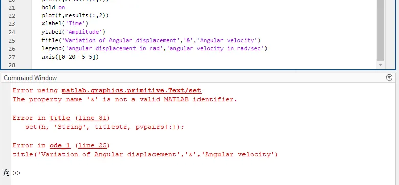
title({'Variation of Angular displacement','&','Angular velocity'})
legend('angular displacement in rad','angular velocity in rad/sec')
axis([0 20 -5 5])

while solving ODE in matlab sub-functions or separate functions can be used to simplify and ease of the procedure.

here I used a separate function called "ode_func" which consists of variables t, theta, b,g,l,m.

the code for sub-function is as follows.

function [dtheta_dt] = ode_func(t,theta,b,g,l,m)


theta1 = theta(1)
theta2 = theta(2)

dtheta1_dt = theta2;
dtheta2_dt = -(b/l)*theta2-(g/l)*sin(theta1);

dtheta_dt = [dtheta1_dt; dtheta2_dt];

end

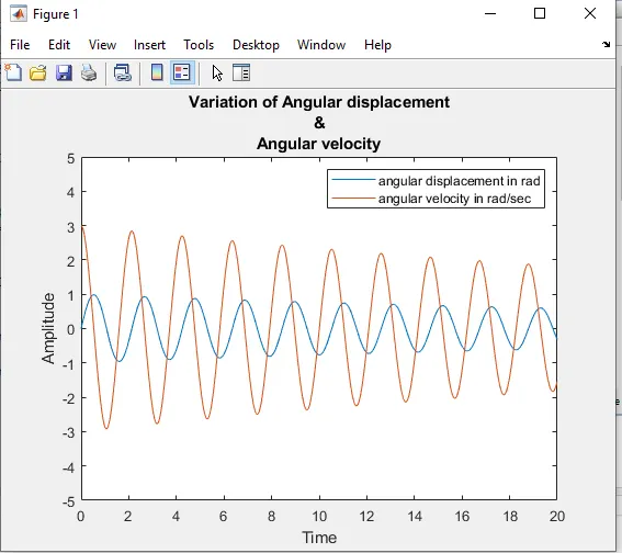
the output of the above code is as below

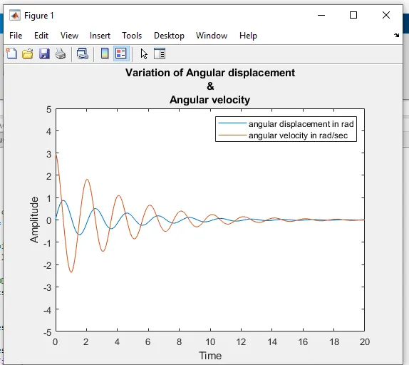
if we change mass value to 0.1 then we will get the following plot.

while giving title to the plot use correct paranthesis, otherwise it shows the following error

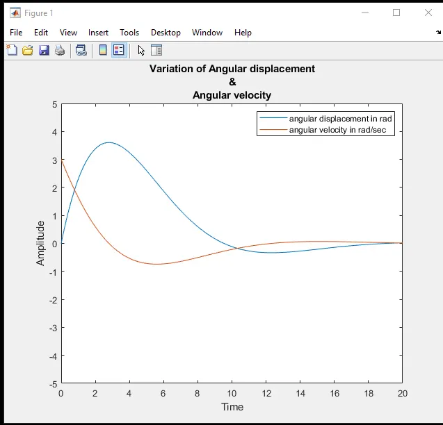
Here the angle is in radians but I write code in degrees then i got a different curve which is a wrong curve.

i corrected the error by changing the code for angle from sind(theta1) to sin(theta1);

the wrong curve is below.

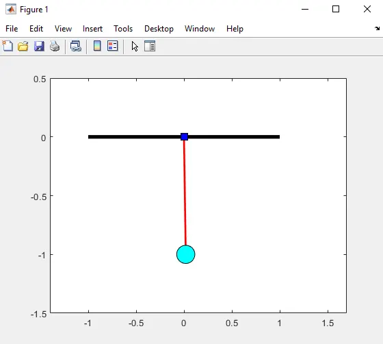
write code to MOTION OF PENDULUM

first fix the position of the pendulum by giving values for x0,y0 and x1,y1

initially at the fixed points are (0,0)

and the points at which the ball of the pendulum hangs are x1= l*sin(theta), y1= -l*cos(theta). here theta is varying according to time interval, so we can use the following formula for ball position.

x1=l*sin(results(i,1));

y1= -l*cos(results(i,1));

here we are repeating the values again and again so use for loop.

the code for motion of the pendulum is as follows

ct=1;
for i=1:length(results(:,1))
    x0=0;
    y0=0;
    plot([-1 1],[0 0],'linewidth',4,'color','k')
    hold on
    
    % position of the ball
    x1 = l*sin(results(i,1));
    y1 = -l*cos(results(i,1));

    % plotting the length of the pendulum
    plot([x0 x1],[y0 y1],'linewidth',2,'color','b')
    
    % fixed end, '-s' indicates square symbol
    plot(x0,y0,'-s','MarkerFaceColor','y','MarkerSize',10)

    % position of the ball, '-o' indicates symbol of circle
    plot(x1,y1,'-o','MarkerFaceColor','g','MarkerSize',20)

    hold off

    axis([-1.4 1.7 -1.5 0.5]);

    pause(0.03);

    ct=ct+1;

end

With this code we can animate the motion of the pendulum. in order to create movie we have to introduce getframe command which gives every frame to a variable.

here we can remove pause command and introduce getframe(gcf) command to animate.

the below given code creates movie

movie(M)
videofile=VideoWriter('motion_of_pendulum')
open(videofile);
writeVideo(videofile,M);
close(videofile);

if we use uncompressed AVI in VideoWriter it creates very large file. so in order to avoid this, skip uncompressed command.

The final code for solving pendulam equation is

clear all
close all
clc

b = 0.05;
g = 9.81;
l = 1;
m = 1;

% intial conditions of angular displacement and angular velocity
theta_0 = [0;3]; % initial displacement =0; intial angular velocity = 3;

% time points
t_span = linspace(0,20,500);

% solve ODE
[t,results] = ode45(@(t,theta)ode_func(t,theta,b,g,l,m),t_span,theta_0);

% plot
figure(1)
plot(t,results(:,1))
hold on
plot(t,results(:,2))
xlabel('Time')
ylabel('Amplitude')
title({'Variation of Angular displacement','&','Angular velocity'})
legend('angular displacement in rad','angular velocity in rad/sec')
axis([0 20 -5 5])

figure(2)
ct=1;
for i=1:length(results(:,1))
    x0=0;
    y0=0;
    plot([-1 1],[0 0],'linewidth',4,'color','k')
    hold on
    x1 = l*sin((results(i,1)));
    y1 = -l*cos((results(i,1)));
    plot([x0 x1],[y0 y1],'linewidth',2,'color','b')
    plot(x0,y0,'-s','MarkerFaceColor','y','MarkerSize',10)
    plot(x1,y1,'-o','MarkerFaceColor','g','MarkerSize',20)
    hold off
    axis([-1.4 1.7 -1.5 0.5]);
    M(ct) = getframe(gcf);
    
    ct=ct+1;
end
movie(M)
videofile= VideoWriter('motion_of_pendulam');
open(videofile);
writeVideo(videofile,M);
close(videofile);

The FINAL OUTPUT IS

1). The graph that shows Variation of Angular displacement & Angular Velocity 2) The plot that shows position of Pendulum

3) The link that contains animation of pendulum motion.

https://drive.google.com/file/d/17zpanHRMAHp36Vo384eMDYIg9zflDKNG/view?usp=sharing