Project 2 - EDA on Vehicle Insurance Customer Data
EDA on VEHICLE INSURANCE DATA
A company has customer data that contains 8 columns of customer details and another table having name customer_policy data contains the policy details of the customer.
The company intends to offer some discount in premium for certain customers. To do that they ask their Data scientist team to get some information. Hence, following tasks DS team decided to perform:
1. Add the column names to both datasets:
i. Column Name for customer details table:
       customer_id,

       Gender,

       age,

       driving licence present,

       region code,

       previously insured,

       vehicle age

       and vehicle damage, in respective order.
ii. Column Name for customer_policy table:
       customer_id,

       annual premium (in Rs),

       sales channel code,

       vintage and response.
2. Checking and Cleaning Data Quality:
i. Null values
- Generate a summary of count of all the null values column wise
- Drop Null values for customer_id because central tendencies for id’s is not feasible.
- Replace all null values for numeric columns by mean.
- Replace all null values for Categorical value by mode.
ii. Outliers
-
Generate a summary of count of all the outliers column wise
-
Replace all outlier values for numeric columns by mean.
(Hint1: for outlier treatment use IQR method as follows:
For example: for a column X calculate Q1 = 25th percentile and Q3 = 75th percentile then IQR = Q3 – Q1 ) then to check outlier, anything lower than a Q1 – 1.5IQR or greater than Q3 + 1.5 IQR would be an outlier
Hint2: For getting percentile value, explore pd.describe() function)
iii. White spaces
- Remove white spaces
iv. case correction(lower or upper, any one)
v. Convert nominal data (categorical) into dummies
for future modeling use if requiredvi. Drop Duplicates (duplicated rows)
3. Create a Master table for future use. Join the customer table and customer_policy table to get a master table using customer_id in both tables.
(Hint: use pd.merge() function)4. Company needs some important information from the master table to make decisions for future growth.They needs following information:
-
i. Gender wise average annual premium
-
ii. Age wise average annual premium
-
iii. Is your data balanced between the genders?
(Hint: Data is balanced if number of counts in each group is approximately same) -
iv. Vehicle age wise average annual premium.
5. Is there any relation between Person Age and annual premium?
Hint: use correlation function (Correlation describes the relationship between two variables).

Correlation coefficient < -0.5           - Strong negative relationship

Correlation coefficient > 0.5            -  Strong positive relationship

0.5 < Correlation coefficient < 0.5   - There is no relationship.
import pandas as pd
import numpy as np
import matplotlib.pyplot as plt
# Loading the data files
df1 = pd.read_csv("customer_details.csv")
df2 = pd.read_csv("customer_policy_details.csv")1. Add the column names to both datasets:
1.(i) Adding columns to customer details table
headers = ['customer_id','Gender','age','driving licence present','region code','previously insured','vehicle age','vehicle damage']

df1.columns=headers

df1.head()| customer_id | Gender | age | driving licence present | region code | previously insured | vehicle age | vehicle damage | |
|---|---|---|---|---|---|---|---|---|
| 0 | 1.0 | Male | 44.0 | 1.0 | 28.0 | 0.0 | > 2 Years | Yes |
| 1 | 2.0 | Male | 76.0 | 1.0 | 3.0 | 0.0 | 1-2 Year | No |
| 2 | 3.0 | Male | 47.0 | 1.0 | 28.0 | 0.0 | > 2 Years | Yes |
| 3 | 4.0 | Male | 21.0 | 1.0 | 11.0 | 1.0 | < 1 Year | No |
| 4 | 5.0 | Female | 29.0 | 1.0 | 41.0 | 1.0 | < 1 Year | No |
1.(ii) Adding columns to customer policy details table
df2.columns=['customer_id','annual premium (in Rs)','sales channel code','vintage','responce']

df2.head()| customer_id | annual premium (in Rs) | sales channel code | vintage | responce | |
|---|---|---|---|---|---|
| 0 | 1.0 | 40454.0 | 26.0 | 217.0 | 1.0 |
| 1 | 2.0 | 33536.0 | 26.0 | 183.0 | 0.0 |
| 2 | 3.0 | 38294.0 | 26.0 | 27.0 | 1.0 |
| 3 | 4.0 | 28619.0 | 152.0 | 203.0 | 0.0 |
| 4 | 5.0 | 27496.0 | 152.0 | 39.0 | 0.0 |
2. Checking and cleaning Data quality
# the column wise count of null values on customer details table
df1_null = df1.isnull()
for i in df1_null.columns.values.tolist():
print(i)
print(df1_null[i].value_counts())
print("")customer_id False 380723 True 386 Name: customer_id, dtype: int64 Gender False 380741 True 368 Name: Gender, dtype: int64 age False 380741 True 368 Name: age, dtype: int64 driving licence present False 380716 True 393 Name: driving licence present, dtype: int64 region code False 380717 True 392 Name: region code, dtype: int64 previously insured False 380728 True 381 Name: previously insured, dtype: int64 vehicle age False 380728 True 381 Name: vehicle age, dtype: int64 vehicle damage False 380702 True 407 Name: vehicle damage, dtype: int64
-
SUMMARY OF NULL VALUES ON CUSTOMER DETAILS TABLE
  customer_id has 386 null values

  Gender has 368 null values

  age has 368 null values

  driving licence present has 393 null values

  region code has 392 null values

  previously insured has 381 null values

  vehicle age has 381 null values

  vehicle damage has 407 null values
# the column wise count of null values on customer policy details table

df2_null = df2.isnull()

for i in df2_null.columns.values.tolist():
    print(i)
    print(df2_null[i].value_counts())
    print("")
customer_id False 380722 True 387 Name: customer_id, dtype: int64 annual premium (in Rs) False 380763 True 346 Name: annual premium (in Rs), dtype: int64 sales channel code False 380709 True 400 Name: sales channel code, dtype: int64 vintage False 380721 True 388 Name: vintage, dtype: int64 responce False 380748 True 361 Name: responce, dtype: int64
-
SUMMARY OF NULL VALUES ON CUSTOMER-POLICY-DETAILS TABLE
 customer_id has 387 null values

 annual premium has 346 null values

 sales channel code has 400 null values

 vintage has 388 null values

 responce has 361 null values
2.i.(b). Droppinf NULL values for customer_id
# Dropping the rows that contains null values of customr_id on customer details table
df1.dropna(subset=['customer_id'], axis=0,inplace=True)

# resetting index because some rows deleted
df1.reset_index(drop = True, inplace = True)
# Dropping the rows that contains null values of customr_id on customer policy details table

df2.dropna(subset=['customer_id'], axis=0,inplace=True)

# resetting index because some rows deleted
df2.reset_index(drop = True, inplace = True)
2.i.(c). Replacing all null values for numeric columns by mean
df1.head()| customer_id | Gender | age | driving licence present | region code | previously insured | vehicle age | vehicle damage | |
|---|---|---|---|---|---|---|---|---|
| 0 | 1.0 | Male | 44.0 | 1.0 | 28.0 | 0.0 | > 2 Years | Yes |
| 1 | 2.0 | Male | 76.0 | 1.0 | 3.0 | 0.0 | 1-2 Year | No |
| 2 | 3.0 | Male | 47.0 | 1.0 | 28.0 | 0.0 | > 2 Years | Yes |
| 3 | 4.0 | Male | 21.0 | 1.0 | 11.0 | 1.0 | < 1 Year | No |
| 4 | 5.0 | Female | 29.0 | 1.0 | 41.0 | 1.0 | < 1 Year | No |
In this table
      age,and region code contains numerical data
      where as driving licence present and previously insured contains categorical data.
# Replacing the NaN values of age by its mean value
df1['age'].fillna(df1['age'].mean(),inplace = True)
# Replacing the NaN values of region code by its mean value
df1['region code'].fillna(df1['region code'].mean(),inplace = True)
df2.head()| customer_id | annual premium (in Rs) | sales channel code | vintage | responce | |
|---|---|---|---|---|---|
| 0 | 1.0 | 40454.0 | 26.0 | 217.0 | 1.0 |
| 1 | 2.0 | 33536.0 | 26.0 | 183.0 | 0.0 |
| 2 | 3.0 | 38294.0 | 26.0 | 27.0 | 1.0 |
| 3 | 4.0 | 28619.0 | 152.0 | 203.0 | 0.0 |
| 4 | 5.0 | 27496.0 | 152.0 | 39.0 | 0.0 |
In this table
       annual premium, sales channel code, and vintage contains numerical data
       where as responce has categorical data
# Replacing the NaN values of annual premium by its mean value
df2['annual premium (in Rs)'].fillna(df2['annual premium (in Rs)'].mean(),inplace = True)
# Replacing the NaN values of sales channel code by its mean value
df2['sales channel code'].fillna(df2['sales channel code'].mean(),inplace = True)
# Replacing the NaN values of vintage by its mean value
df2['vintage'].fillna(df2['vintage'].mean(),inplace = True)
2.i.(d) Repalcing categorical null values by its mode.
# it replaces the null values with the value which exist maximum no of times i.e. mode
df1['driving licence present'].fillna (df1['driving licence present'].mode()[0], inplace=True)

# it replaces the null values with the value which exist maximum no of times i.e. mode
df1['previously insured'].fillna (df1['previously insured'].mode()[0], inplace=True)
# it replaces the null values with the value which exist maximum no of times i.e. mode
df2['responce'].fillna(df2['responce'].mode()[0], inplace=True)2.(ii) OUTLIERS
2.ii.(a). Summary of Count of Outliers
In customer details table we need to calculate outliers for columns age and regional code.others are non-numerical columns so ignore them
# this is the function to boxplot for easy visualisation of outliers..

def plot_boxplot(df,ft):
    df.boxplot(column=[ft])
    plt.grid(False)
    plt.show()
plot_boxplot(df1,'age') 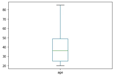
plot_boxplot(df1,'region code') 
    from the above boxplot figures we can easily understand there are no outliers for customer details table.
    lets see summary of the outliers for the customer details..
# this functions finds outliers if present by IQR method..
def finding_outliers(df):
q1 = df.quantile(0.25)
q3 = df.quantile(0.75)
iqr = q3-q1
outlier = df[((df<(q1-1.5*iqr)) | (df>(q3+1.5*iqr)))]
return outlieroutliers = finding_outliers(df1['age'])
print('Number of outliers :',len(outliers))
print('Maximum outlier value :',outliers.max())
print('Minimum outlier value :',outliers.min())Number of outliers : 0 Maximum outlier value : nan Minimum outlier value : nan
outliers = finding_outliers(df1['region code'])

print('Number of outliers :',len(outliers))
print('Maximum outlier value :',outliers.max())
print('Minimum outlier value :',outliers.min())
Number of outliers : 0 Maximum outlier value : nan Minimum outlier value : nan
from the above results we can conclude that customer details table doesn't have outliers..
Finding outliers for customer policy details..
plot_boxplot(df2,'annual premium (in Rs)') 
plot_boxplot(df2,'sales channel code') 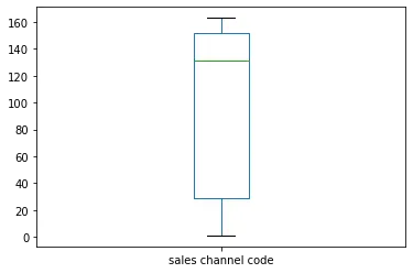
plot_boxplot(df2,'vintage') 
From the above boxplot graphs we can conclude that only column annual premium has outliers.. lets find the summary of the outliers..
outliers = finding_outliers(df2['annual premium (in Rs)'])

print('Number of outliers :',len(outliers))
print('Maximum outlier value :',outliers.max())
print('Minimum outlier value :',outliers.min())
Number of outliers : 10332 Maximum outlier value : 540165.0 Minimum outlier value : 61858.0
outliers = finding_outliers(df2['sales channel code'])

print('Number of outliers :',len(outliers))
print('Maximum outlier value :',outliers.max())
print('Minimum outlier value :',outliers.min())
Number of outliers : 0 Maximum outlier value : nan Minimum outlier value : nan
outliers = finding_outliers(df2['vintage'])

print('Number of outliers :',len(outliers))
print('Maximum outlier value :',outliers.max())
print('Minimum outlier value :',outliers.min())
Number of outliers : 0 Maximum outlier value : nan Minimum outlier value : nan
2.ii.(b).Replacing the outliers with mean values
def replace_outlier(df):
    q1 = df.quantile(0.25)
    q3 = df.quantile(0.75)
    iqr = q3-q1
    upper = df[~(df>(q3+1.5*iqr))].max()
    lower = df[~(df<(q1-1.5*iqr))].min()
    df = np.where(df>upper,df.mean(),np.where(df<lower,df.mean(),df))
    return df
df2['annual premium (in Rs)'] = replace_outlier(df2['annual premium (in Rs)'])2.(iii). Remove white spaces
df1.apply(lambda x: x.str.strip() if x.dtype=='object' else x)| customer_id | Gender | age | driving licence present | region code | previously insured | vehicle age | vehicle damage | |
|---|---|---|---|---|---|---|---|---|
| 0 | 1.0 | Male | 44.0 | 1.0 | 28.0 | 0.0 | > 2 Years | Yes |
| 1 | 2.0 | Male | 76.0 | 1.0 | 3.0 | 0.0 | 1-2 Year | No |
| 2 | 3.0 | Male | 47.0 | 1.0 | 28.0 | 0.0 | > 2 Years | Yes |
| 3 | 4.0 | Male | 21.0 | 1.0 | 11.0 | 1.0 | < 1 Year | No |
| 4 | 5.0 | Female | 29.0 | 1.0 | 41.0 | 1.0 | < 1 Year | No |
| ... | ... | ... | ... | ... | ... | ... | ... | ... |
| 380718 | 381105.0 | Male | 74.0 | 1.0 | 26.0 | 1.0 | 1-2 Year | No |
| 380719 | 381106.0 | Male | 30.0 | 1.0 | 37.0 | 1.0 | < 1 Year | No |
| 380720 | 381107.0 | Male | 21.0 | 1.0 | 30.0 | 1.0 | < 1 Year | No |
| 380721 | 381108.0 | Female | 68.0 | 1.0 | 14.0 | 0.0 | > 2 Years | Yes |
| 380722 | 381109.0 | Male | 46.0 | 1.0 | 29.0 | 0.0 | 1-2 Year | No |
NOTE: The customer policy details tables containls all the columns of float type only.so no need to remove spaces
2.(iv). Case Correction
convert all the characters to upper case.
df1.apply(lambda x: x.str.upper() if x.dtype=='object' else x)| customer_id | Gender | age | driving licence present | region code | previously insured | vehicle age | vehicle damage | |
|---|---|---|---|---|---|---|---|---|
| 0 | 1.0 | MALE | 44.0 | 1.0 | 28.0 | 0.0 | > 2 YEARS | YES |
| 1 | 2.0 | MALE | 76.0 | 1.0 | 3.0 | 0.0 | 1-2 YEAR | NO |
| 2 | 3.0 | MALE | 47.0 | 1.0 | 28.0 | 0.0 | > 2 YEARS | YES |
| 3 | 4.0 | MALE | 21.0 | 1.0 | 11.0 | 1.0 | < 1 YEAR | NO |
| 4 | 5.0 | FEMALE | 29.0 | 1.0 | 41.0 | 1.0 | < 1 YEAR | NO |
| ... | ... | ... | ... | ... | ... | ... | ... | ... |
| 380718 | 381105.0 | MALE | 74.0 | 1.0 | 26.0 | 1.0 | 1-2 YEAR | NO |
| 380719 | 381106.0 | MALE | 30.0 | 1.0 | 37.0 | 1.0 | < 1 YEAR | NO |
| 380720 | 381107.0 | MALE | 21.0 | 1.0 | 30.0 | 1.0 | < 1 YEAR | NO |
| 380721 | 381108.0 | FEMALE | 68.0 | 1.0 | 14.0 | 0.0 | > 2 YEARS | YES |
| 380722 | 381109.0 | MALE | 46.0 | 1.0 | 29.0 | 0.0 | 1-2 YEAR | NO |
2.(v). Convert nominal data into dummy variables
Indicator Variable (or Dummy Variable)
What is an indicator variable?
An indicator variable (or dummy variable) is a numerical variable used to label categories. They are called 'dummies' because the numbers themselves don't have inherent meaning.
Why we use indicator variables?
We use indicator variables so we can use categorical variables for regression analysis in the later modules.Example
We see the column "vehicle damage" has two unique values: "Yes" or "No". Regression doesn't understand words, only numbers. To use this attribute in regression analysis, we convert "vehicle damage" to indicator variables.
We will use pandas' method 'get_dummies' to assign numerical values to different categories of vehicle damage.
# Creating dummy variable for vehicle damage

dummy_variable_1 = pd.get_dummies(df1["vehicle damage"])

dummy_variable_1.head()| No | Yes | |
|---|---|---|
| 0 | 0 | 1 |
| 1 | 1 | 0 |
| 2 | 0 | 1 |
| 3 | 1 | 0 |
| 4 | 1 | 0 |
# Changing the column names for dummy variable

dummy_variable_1.rename(columns={'No':'vehicle-damage-No', 'Yes':'vehicle-damage-Yes'}, inplace=True)

dummy_variable_1.head()| vehicle-damage-No | vehicle-damage-Yes | |
|---|---|---|
| 0 | 0 | 1 |
| 1 | 1 | 0 |
| 2 | 0 | 1 |
| 3 | 1 | 0 |
| 4 | 1 | 0 |
# merge data frame "df1" and "dummy_variable_1"
df1 = pd.concat([df1, dummy_variable_1], axis=1)

# drop original column "vehicle damage" from "df1"
df1.drop("vehicle damage", axis = 1, inplace=True)
similary we can create a dummy variable for gender if needed.
2.(vi). Drop Duplicates
# Dropping duplicates from customer details table

df1.drop_duplicates(inplace=True)


# Dropping duplicates from customer policy details table

df2.drop_duplicates(inplace=True)
3. Merging the data sets.
master_data = pd.merge(df1,df2,on='customer_id')

master_data| customer_id | Gender | age | driving licence present | region code | previously insured | vehicle age | vehicle-damage-No | vehicle-damage-Yes | annual premium (in Rs) | sales channel code | vintage | responce | |
|---|---|---|---|---|---|---|---|---|---|---|---|---|---|
| 0 | 1.0 | Male | 44.0 | 1.0 | 28.0 | 0.0 | > 2 Years | 0 | 1 | 40454.0 | 26.0 | 217.0 | 1.0 |
| 1 | 2.0 | Male | 76.0 | 1.0 | 3.0 | 0.0 | 1-2 Year | 1 | 0 | 33536.0 | 26.0 | 183.0 | 0.0 |
| 2 | 3.0 | Male | 47.0 | 1.0 | 28.0 | 0.0 | > 2 Years | 0 | 1 | 38294.0 | 26.0 | 27.0 | 1.0 |
| 3 | 4.0 | Male | 21.0 | 1.0 | 11.0 | 1.0 | < 1 Year | 1 | 0 | 28619.0 | 152.0 | 203.0 | 0.0 |
| 4 | 5.0 | Female | 29.0 | 1.0 | 41.0 | 1.0 | < 1 Year | 1 | 0 | 27496.0 | 152.0 | 39.0 | 0.0 |
| ... | ... | ... | ... | ... | ... | ... | ... | ... | ... | ... | ... | ... | ... |
| 380331 | 381105.0 | Male | 74.0 | 1.0 | 26.0 | 1.0 | 1-2 Year | 1 | 0 | 30170.0 | 26.0 | 88.0 | 0.0 |
| 380332 | 381106.0 | Male | 30.0 | 1.0 | 37.0 | 1.0 | < 1 Year | 1 | 0 | 40016.0 | 152.0 | 131.0 | 0.0 |
| 380333 | 381107.0 | Male | 21.0 | 1.0 | 30.0 | 1.0 | < 1 Year | 1 | 0 | 35118.0 | 160.0 | 161.0 | 0.0 |
| 380334 | 381108.0 | Female | 68.0 | 1.0 | 14.0 | 0.0 | > 2 Years | 0 | 1 | 44617.0 | 124.0 | 74.0 | 0.0 |
| 380335 | 381109.0 | Male | 46.0 | 1.0 | 29.0 | 0.0 | 1-2 Year | 1 | 0 | 41777.0 | 26.0 | 237.0 | 0.0 |
4. getting required data for decisions
4.(i). Gender wise average annual premium
gender_data = master_data.groupby('Gender')['annual premium (in Rs)'].mean()

gender_data
Gender Female 29273.474247 Male 29323.022594 Name: annual premium (in Rs), dtype: float64
# plots a linear graph

gender_data.plot() 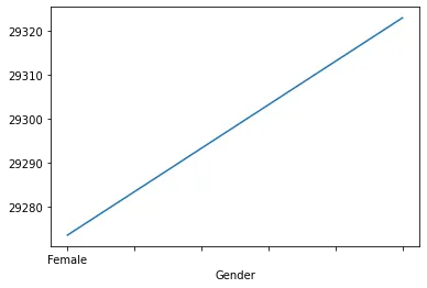
# plotting a bar graph

gender_data.plot.bar(title='Gender vs average annual premium') 
4.(ii). age wise average annual premium
age_data = master_data.groupby('age')['annual premium (in Rs)'].mean()

age_data
age
20.0 26342.073517
21.0 29751.791916
22.0 29946.848634
23.0 29838.344763
24.0 30125.557096
...
81.0 29287.910702
82.0 36480.586199
83.0 28995.818172
84.0 35440.818182
85.0 26637.454525
Name: annual premium (in Rs), Length: 67, dtype: float64
# showing the results on a linear graph

age_data.plot(xlabel="age",ylabel="annual premium(in Rs)",title="Age vs Average annual premium") 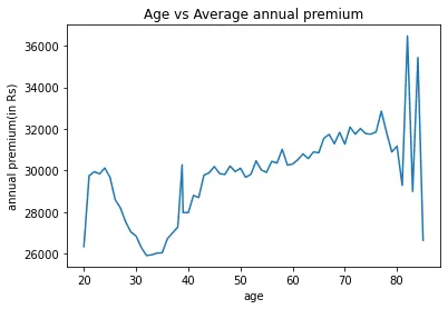
# plotting a bar graph

age_data.plot.bar() 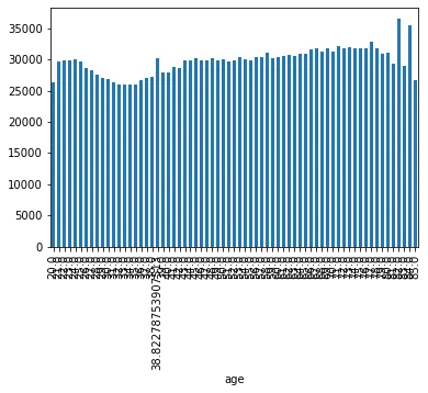
4.(iii). Checking Balanced between gender or not..
master_data.groupby('Gender').count()| customer_id | age | driving licence present | region code | previously insured | vehicle age | vehicle-damage-No | vehicle-damage-Yes | annual premium (in Rs) | sales channel code | vintage | responce | |
|---|---|---|---|---|---|---|---|---|---|---|---|---|
| Gender | ||||||||||||
| Female | 174485 | 174485 | 174485 | 174485 | 174485 | 174309 | 174485 | 174485 | 174485 | 174485 | 174485 | 174485 |
| Male | 205484 | 205484 | 205484 | 205484 | 205484 | 205279 | 205484 | 205484 | 205484 | 205484 | 205484 | 205484 |
- summary
  The ratio between male and female is approximately 1. (1.177)
  Here the data between Gender is approximately same.. so the data is balanced..
4.(iv). Vehicle age wise average annual premium
vehicle_age = master_data.groupby('vehicle age')['annual premium (in Rs)'].mean()

vehicle_age
vehicle age 1-2 Year 29099.066738 < 1 Year 29188.150594 > 2 Years 32943.540830 Name: annual premium (in Rs), dtype: float64
vehicle_age.plot() # linear graph 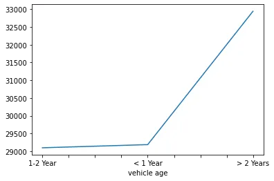
vehicle_age.plot.bar() # bar graph 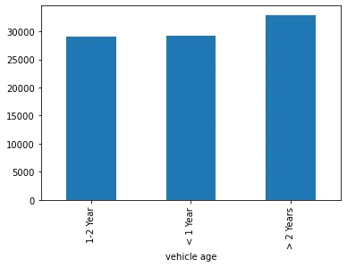
5. Correlation between age and annual premuim
Pearson Correlation
The Pearson Correlation measures the linear dependence between two variables X and Y.
The resulting coefficient is a value between -1 and 1 inclusive, where:
- 1: Perfect positive linear correlation.
- 0: No linear correlation, the two variables most likely do not affect each other.
- -1: Perfect negative linear correlation.
-
Correlation coefficient < -0.5 - Strong negative relationship
-
Correlation coefficient > 0.5 - Strong positive relationship
-
-0.5 < Correlation coefficient < 0.5 - There is no relationship.
# finding the correlation coefficient in pandas

master_data['age'].corr(master_data['annual premium (in Rs)'])
0.0506575892861754
# Matrix form of correlation
master_data[['age','annual premium (in Rs)']].corr()| age | annual premium (in Rs) | |
|---|---|---|
| age | 1.000000 | 0.050658 |
| annual premium (in Rs) | 0.050658 | 1.000000 |
Summary
Since the Pearson coefficient lies between 0.5 and -.5, So no relation between age and annual premium