Week 3 - Solving second order ODEs

• aim: To write a programme that will solve the ordinary differential eqn.

• the equation of motion of simple pendulum is written below with damping.

in engineering ODE is used to describe transient behaviour of a system.a example is simple pendulum the following is the 2nd order ode of simple pendulum.the way the pendulum moves depends on newtons 2nd law.

d²θ/dt²+b/m(dϴ/dt)+(g/L)sinθ=0.......................eqn (i)

b=damping cofficient=0.05

L=length of pendelum=1m

m=mass of pendulum=1kg

g=acceleration due to gravity=9.8m/sec

lets solve the 2nd order above eqn 1 we get theta1 and theta2

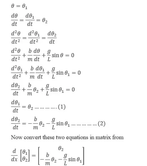
eqn 1 and eqn 2nd can be written in the matrix form .

points to be remember about ode45 solver

• A numerical ODE solver is used as the main tool to solve the ODE's. The matlab function ode45 will be used. The important thing to remember is that ode45 can only solve a first order ODE.

• we can use ode45 solver to solve the above ode function in our matlab programme.
• steps of the programme.

• first of all we are going to make a function that will calculate the value of theta 1 and theta 2 whwn we pass some inputs to it.after getting the values of theta 1 and theta 2 ,we are going to call it from main programme.
• let me write down the function below.
• function[dtheta_dt]=ode_func(t,theta ,b,g,l,m)
  theta1=theta(1);
  theta2=theta(2);
  dtheta1_dt=theta2;
  dtheta2_dt=(-b/m)*theta2-(g/l)*sin(theta1);
  dtheta_dt=[dtheta1_dt;dtheta2_dt];
  end
• our next step is to write main programme

% write a programme to solve ode for a pendelum
clear all
close all
clc
%intial condtions/inputs
%b=damping cofficient
b=0.05; % semicolans ; used here for surpressing the results from damping cofficient
%m=mass of simple pendelum
m=1;
%acc due to gravity 'g'
g=9.81;
%l=length of pendelum
l=1;
%we have 2 ode's one is for displacement and other is for velocity
%intial condtions
%theta_Z=[0;5];
theta_z=[0 ;5];
%to integrate the above solution value we have to define time value
t_span =linspace(0,20,500);
%now we are going to solve ode
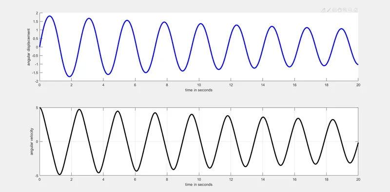
[t,results]=ode45(@(t,theta) ode_func(t,theta,b,g,l,m),t_span,theta_z);
%ploting for tracing of angular velocity and angular displacement
subplot(2,1,1)
hold on;
plot(t,results(:,1),'b','linewidth',3);
xlabel('time in seconds');
ylabel('angular displacement');
subplot(2,1,2)
hold off
plot(t,results(:,2),'k','linewidth',3);
xlabel('time in seconds');
ylabel('angular velocity');
grid on;
%below code will help is for animation

ct=1; %ct represents ,actually each and every frame
for i=1:length(results(:,1))
x0=0;
y0=0;
x1=l*sin(results(i,1));
y1=-l*cos(results(i,1));
subplot(2,2,2)
plot([-1 1],[0 0],'linewidth',6,'color','g');
axis([-2 2 -2 2]);
line([x0 x1],[y0 y1],'linewidth',2,'color','b');
hold on;
plot(x0,y0,'o','markersize',3,'markerfacecolor','y');
plot(x1,y1,'o','markersize',20,'markerfacecolor','r');
title('damping of simple pendulum');
legend('support rod','length 0f pendulum','fixedpoint','bob of pendulum');
pause(0.0);
grid on;
hold off;
M(ct)=getframe(gcf);
ct=ct+1;
end

%code to animate the motion
movie(M)
videofile=videowriter('odesimplependulum.avi','uncompressed AVI');
open(videofile)
writevideo(videofile,M)
close(videofile)