Week 3 - Solving second order ODEs

Skill-lync assignment 3

Aim: The objective of this assignment is to create a Python code that simulate the movement of a simple pendulum and present it as an animation. The pendulum movement is to be coded as the solution of an ordinary differential equation.

Problem statement: A simple pendulum is one of the simplest processes that can be modelled using ordinary differential equations (ODEs). The code to be created is to express the main ODE as a matrix of first order ODEs that is to be solved to get the displacements & velocities. The various parameters and boundary conditions for these ODEs are listed below.

• L1 (pendulum length): 1 m
• m1 (pendulum mass): 1 kg
• b1 (damping coefficient): 0.05
• g1 (gravitational acceleration): 9.80665 m/s²
• t1 (time period): 20 sec
• theta1_init (initial angular displacement): 0 rad
• theta2_init (initial angular velocity): 3 rad/s

Theory: The movement of a simple pendulum can be defined by the following second order ODE.

, or

θ̎ + (b/m)θ̍ + (g/L)Sinθ = 0 (1)

Angular displacement can be expressed by θ₁.

Angular velocity can be expressed by θ₂.

θ₂ = θ₁̍ (2)

Using (2) in (1),

θ₁̎ + (b/m)θ₁̍ + (g/L)Sinθ₁ = 0

θ₂̍ + (b/m)θ₂ + (g/L)Sinθ₁ = 0

θ₂̍ = -(b/m)θ₂ – (g/L)Sinθ₁ (3)

Thus, the first order differential equations of (2) & (3) can be expressed as a 2 X 1 matrix, as shown below.

Thus, integrating these values with respect to time will give the full range of angular displacements and velocities throughout the specified time period.

Procedure: The code is constructed with the following sequence of steps.

1. After opening the Sublime text editor, the first lines of code are used to import the math, matplotlib, numpy and scipy modules, as shown in the screenshot below.

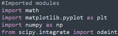
Figure 1: Python modules used in the code

2. Next, the pendulum parameters are defined with their respective values.
3. The initial boundary conditions of angular displacement & velocity are then defined. These values are then used to define an array for initial conditions, as shown below.

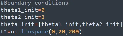
Figure 2: Boundary conditions for ODEs

4. The time period is defined as a linearly spaced array with its respective time period and number of intervals using the np.linspace command.
5. A function pend is defined to define the ODEs for variables theta1 & theta2, as shown in the screenshot below.

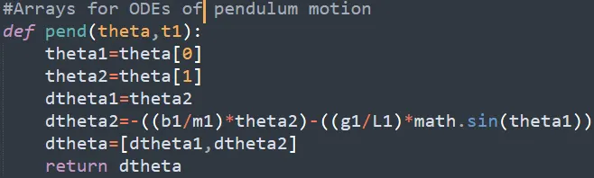Figure 3: Definition of ODEs and variables

6. The full range of values for the array containing the variables theta1 & theta2 are computed by using the odeint command to solve the ODEs defined in the function earlier.
7. These values are then used to plot the displacement/velocity vs. time curve graph, which is then saved to the local directory.
8. The variable theta1 is used to generate the images of the pendulum. The pendulum is modelled as a straight line between the pivot point and the end point of the pendulum. The coordinates of the pivot point are defined in the following manner.

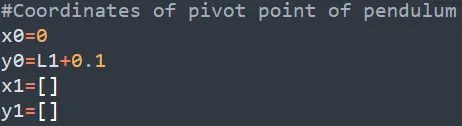
Figure 4: Coordinates for animating pendulum

9. A for loop is defined to compute the end point of the pendulum, as well as generate the animation. The loop is shown below.

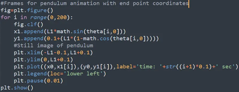Figure 5: Loop for generating animation images

10. The images are combined to create a gif animation of the pendulum.

Results: The complete code for the pendulum animation is listed below.

#Imported modules
import math
import matplotlib.pyplot as plt
import numpy as np
from scipy.integrate import odeint

#Pendulum parameters
L1=1
m1=1
b1=0.05
g1=9.80665

#Boundary conditions
theta1_init=0
theta2_init=3
theta_init=[theta1_init,theta2_init]
t1=np.arange(0,20.1,0.1)

#Arrays for ODEs of pendulum motion
def pend(theta,t1):
	theta1=theta[0]
	theta2=theta[1]
	dtheta1=theta2
	dtheta2=-((b1/m1)*theta2)-((g1/L1)*math.sin(theta1))
	dtheta=[dtheta1,dtheta2]
	return dtheta

#Array for solution to ODEs
theta = odeint(pend,theta_init,t1)

#Plot of displacement and velocity history
plt.figure()
plt.plot(t1,theta[:,0],label='displacement (theta1)')
plt.plot(t1,theta[:,1],label='velocity (theta2)')
plt.xlabel('time (sec)')
plt.legend(loc='best')
plt.savefig('displacement_velocity.png')

#Coordinates of pivot point of pendulum
x0=0
y0=L1+0.1
x1=[]
y1=[]

#Frames for pendulum animation with end point coordinates
fig=plt.figure()
for i in range(0,200):
	fig.clf()
	x1.append(L1*math.sin(theta[i,0]))
	y1.append(0.1+(L1*(1-math.cos(theta[i,0]))))
	#Still image of pendulum
	plt.xlim(-L1-0.1,L1+0.1)
	plt.ylim(0,L1+0.1)
	plt.plot((x0,x1[i]),(y0,y1[i]),label='time: '+str((i+1)*0.1)+' sec')
	plt.legend(loc='lower left')
	plt.pause(0.01)
plt.show()

While the pendulum animation shows elongation & shrinkage caused by the unequal sizes of the x & y axes that is not realistic, it accurately captures the oscillations of the pendulum as well as the subtle dampening of motion. The displacement & velocity plot shown below also capture this detail.

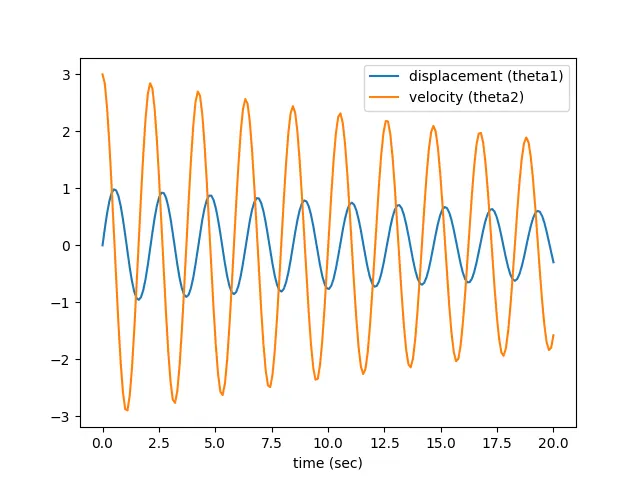Figure 6: Plot of displacement and velocity histories

The plot also shows the phase difference between these two values, such that the peaks/troughs of one of these parameters coincides with the zero value of the other.

Conclusion: The Python code has been properly built to accurately animate the motion of a pendulum. While the animation itself is not perfect, it does capture the variation of parameters with time very well.