Week 3 - Solving second order ODEs
AIM:
To solve an ODE & use the calculated information to animate the motion of the pendulum using matlab.
INTRODUCTION:
* It have many forms & utilized often before the digital age.
* A simple pendulum is consist of a point mass suspended on a string that has negligible mass.
* It will swing back & forth at a regular period & frequency.
* Ordinary differential equation is a differential equation containing one or more functions of one independent variable & the derivates of those functions.
EXPLANATION:
GIVEN:
Gravity(g) = 9.81 m/s^2
Mass of the ball(m) = 0.1 kg
Damping coefficient(b) = 0.05
Length of the pendulum(l) =1 m
Simulation motion =0-20 sec
Angular displacement = 0,
Anmgular velocity = 3 rad/sec @ time, t=0.
CODE:
clear all
close all
clc
%parameters
b = 0.05
g = 9.81
l = 1
m = 0.1
%initial condition
% It is required to provide value for displacement and velocity for solving 1st ode
% initial displacement of the pendulum is 0
% initial velocity is 3 m/s.
theta_0 = [0;5];
% time intervals
t_span = linspace(0,20,500);
%solve ODE
[t,results] = ode45(@(t,theta) ODE_func(t,theta,b,g,l,m) , t_span, theta_0);
outcome = results(:,1);
* Time interval is the time span for which our pendulum shows permanent motion & generate results by using command ode45 which is an inbuilt function for solving differential equations.
*Outcome is nothing but the results following 1st column.
*ODE_function command here is hyperlinked code written to solve differential equation.
ODE_function code:
function [dtheta_dt] = ODE_func(t,theta,b,g,l,m)
theta1 = theta(1)
theta2 = theta(2)
dtheta1_dt = theta2;
dtheta2_dt = -(b/m)*theta2 -(g/l)*sin(theta1);
dtheta_dt = [dtheta1_dt; dtheta2_dt];
end
We solved here 2nd order differential equations & encoded them into code.
% Contor_command
ct = 1;
for i = 1:length(outcome)
pos =outcome(i);
%points
x0 = 0;
y0 = 0;
% max condition
x1 = l*sin(pos);
y1 = -l*cos(pos);
%plotting
plot([x0 x1],[y0 y1],x1,y1,'g.','markersize',15,'linewidth',2)
axis([-1.5 1.5 -1.5 0.5])
grid on
M(ct) = getframe(gcf);
ct = ct+1;
end
contor command is used to change loop irretation after every motion X=0 & Y=0. Using trignometry function we can generate permanent motion of the pendulum & maximum position of the pendulum motion. In this using the marker command to attach a bounce to pendulum string.
%Animation
movie(M)
videofile = VideoWriter('second_order_pendulum');
open(videofile)
writeVideo(videofile,M)
close(videofile)
%plotting
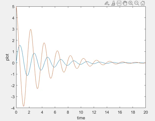
plot(t, results(:,1))
plot(t, results(:,2))
xlabel('time')
ylabel('plot')
axis([0 23 -2.5 2.5])
legend('Angular displacement/time','Angular displacement/time')
* Before starting the program code, it is important to start with clear all, close all, clc.
* Clear all - removes data from the workspace, freeing up system memory
* Close all - deletes the current figure
* Clc - clears all input & output from the window command display, giving a clean screen.
* To define the inputs & variables. The damping coefficient, gravity, length of the pendulum, mass of the ball have been defined.
* To define the initial conditions, the angular displacement & angular velocity have been defined & also be defined the time span.
* To solve the ODE, Ode45 was used. It is a function in matlab that solves ordinary or partial differential equations using a numerical method. The function ode45 takes 3inputs. The 3inputs are the functions to be integrated, the time span and the initial condition.[t, results] means that the results that have been calculated with respect to time.
* After calculating the results, a graph has to be plotted, the graph contain two plots. One for angular displacement with respect to time & one for angular velocity with respect for time. The legend for the graph & the axis labels have been defined.
* [x0 x1 y0 y1] and their corresponding relations are entered to form a string of the pendulum. Markersize was command used to form the mass of the pendulum.
* Finally the code is to create a movie of the animation of the robotic arm, the movie command was used. The videowriter command was used to assign the video format. The open command was used to open the videofile. The writevideo command was used to write the videofile with plots frames. Finally the close command was used to close the videofile.
OUTPUT:
CONCLISION:
The x0,y0,x1,y1 values are given below,
x0 = 0
y0 = 0
x1 = -0.0113
y1 = -0.9999
%ANIMATION OF THE PENDULUM:
Here is the link for the animation video.
https://drive.google.com/file/d/1GuIjgUsATm1CSNZ8xtl-ooULrtjDQmgn/view?usp=sharing