Week 3 - Solving second order ODEs

Transitional Behaviour of a simple pendulum:

A simple pendulum consists of a mass m hanging from a string of length L and fixed at a pivot point P. When displaced to an initial angle and released, the pendulum will swing back and forth with periodic motion.

ODE defining the behaviour of the simple pendulum:

The following is a 2nd order ODE

`(d^2theta)/(dt^2) + b/m (d theta)/(dt) + g/L sintheta =0`

Where b is the damping coefficient

m is the mass of the bob

L is the length of the pendulum

`theta` is angle made by the pendulum with reference to the vertical.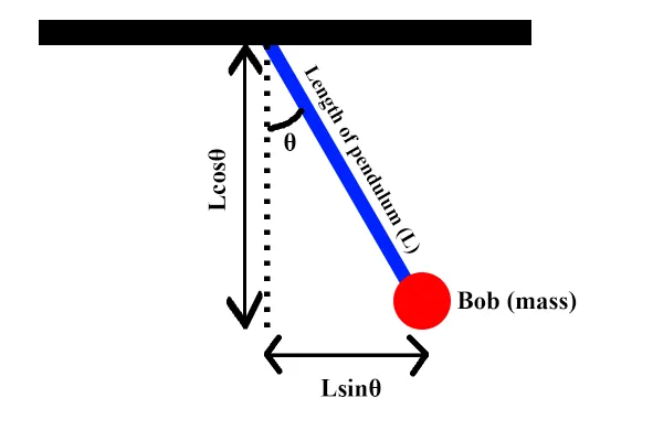

Inputs:

Length of pendulum L= 1m.

Damping coefficient b=0.05.

Mass of bob m = 1kg.

Acceleration due to gravity g = 9.81m/s^2

Initial conditions:

Initial angular displacement = 0.

Initial Angular velocity = 3 rad/sec.

Simulation time = 0 to 20 sec.

Code:

import math
import matplotlib. pyplot as plt
import numpy as np
from scipy. integrate import odeint

def model(theta, t, b, g, l, m):
    theta1 = theta[0]
    theta2 = theta[1]
    dtheta1_dt = theta2
    dtheta2_dt = -(b/m)*theta2 - (g/l)*math.sin(theta1)
    dtheta_dt = [dtheta1_dt, dtheta2_dt]
    return dtheta_dt

#parameters
b = 0.05
g = 9.81
l = 1
m = 0.1

# initial condition
theta_0 = [0,3]
# time points
time = np.linspace(0,20,300)
# Solving ODE
theta = odeint(model, theta_0,time, args = (b, g, l, m))


#plotting
plt. figure(1)
plt.plot(time, theta[:, 0] , 'b-',Label = r'$\frac{d\theta_1}{dt}=\theta_2$')
plt. plot(time, theta[:, 1], 'r--', label = r'$\frac{d\theta_2}{dt} = -\frac{b}{m}\theta_2 - \frac{g}{l}sin\theta_1$')
plt.xlabel ('Time')
plt.ylabel('Plot')
plt. legend (loc ='best')
plt.show()

#animation
ang_disp = []
ang_vel = []

for j in range(0,len(theta)):
    ang_disp.append(theta[j,0])
    ang_vel.append(theta[j,1])

# Simulating the simple pendulum
x0 = 0
y0 = 0
# creating a for loop to simulate the simple pendulum
ct = 1
for i in range (0, len(time)) :
    THETA = Angular_displacement [i]
    x1 = -l*math.sin(THETA)
    y1 = -l*math.cos(THETA)
    filename = '%05d' %ct
    ct = ct + 1

    plt.figure (2)
    plt.plot([-0.5, 0.5], [0, 0] , color ='dimgrey', linewidth = 10)
    plt.plot([x0, x1], [y0, y1], color = 'r')
    plt.plot(x1, y1, marker = 'o',markerfacecolor = 'k' ,markeredgecolor = 'k', markersize = 15)
    plt.xlim([-1,1])
    plt.ylim([-2,0])
    plt.savefig(filename)
    plt. clf()

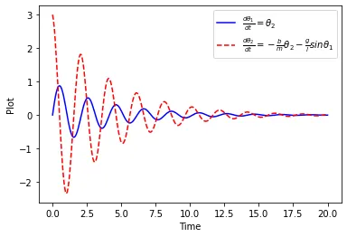
Plot:

Link to animation video:

https://drive.google.com/file/d/1UaAU2XjxZ9gaiSjtPRPrabk3NRJghjlO/view?usp=sharing

Conclusion:

The ODE is solved using Python and simulation of Transient behaviour of a simple pendulum is done.