Solving second order ODEs

AIM:

To write a program that solves the Second order ODE.

To write a program in Matlab that will simulate the pendulum motion.

THEORY:

A simple pendulum is one which can be considered to be a point mass suspended from a string or rod of negligible mass.

In Engineering, ODE is used to describe the transient behavior of a system. A simple example is a pendulum.The way the pendulum moves depends on the Newtons second law. When this law is written down, we get a second order Ordinary Differential Equation that describes the position of the "ball" w.r.t time.

Mathematical Equation

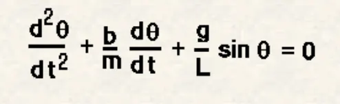
In the above equation,

g = gravity in m/s2,

L = length of the pendulum in m,

m = mass of the ball in kg,

b=damping coefficient

MATLAB code:

%Solving second order ODE and simulate the animation of pendulum
clear all
close all
clc

%Inputs
b = 0.05;   %Damping Coefficient
g = 9.81;   %Gravity constant
l = 1;      %Length of the pendulum
m = 0.1;    %mass

%Initial conditions for defining ODE
theta_0 = [0;3];   %where 0 is initial displacement and 5 is initial velocity

%time points for pendulum oscillation i.e from 0 to 20 sec
t_span = linspace(0,20,150);

%to solve ODE
[t , results] = ode45(@(t,theta)ode_func(t,theta,b,g,l,m),t_span,theta_0)

%Plot 
figure (1)
plot(t,results(:,1),'color','r')
hold on
plot(t,results(:,2),'color','b')
title('Harmonic Motion of Pendulum')
legend('Angular displacement (red)','Angular velocity (blue)')
ylabel('Plot')
xlabel('time')

%Animation
%for loop
%Before loop a counter value has to be defined
ct = 1;
for i = 1:length(results(:,1))
    x_start = 0
    y_start = 0
    x_end = l*sin(results(i,1))
    y_end = -l*cos(results(i,1))
    
    %Plotting the animation
    figure (2)
    plot([-1,1],[0,0],'linewidth',5)
    hold on
    plot([x_start x_end],[y_start y_end],'linewidth',3)
    hold on
    
    plot(x_end,y_end,'o','markersize',20,'markerFacecolor','y')
    title('Animation of transient behaviour of a Pendulum')
    axis([-1.5 1.5 -1.5 1.5])
    pause(0.03)
    hold off
    
    M(ct) = getframe(gcf)
    ct = ct + 1
end

%Animation of pendulum
movie(M)
videofile = VideoWriter('Pendulum Animation.avi','uncompressed avi')
open (videofile)
writeVideo(videofile,M)
close(videofile)

EXPLANATION of Code:

Before writing any code

• clear all

  close all

  clc

  has to be done to clear the workspace,system memory and to start the fresh code.

• We have to define inputs i.e damping coefficient,gravity constant,length and mass.
• In next step we have defined initial velocity and displacement and also time span is defined.
• By using ode45 command ODE function is introduced.
• Using plot command velocity and displacement is plotted.
• Using loop command we get the animation by stiching the graphs of pendulum which were at different positions and is saved.

Plot:

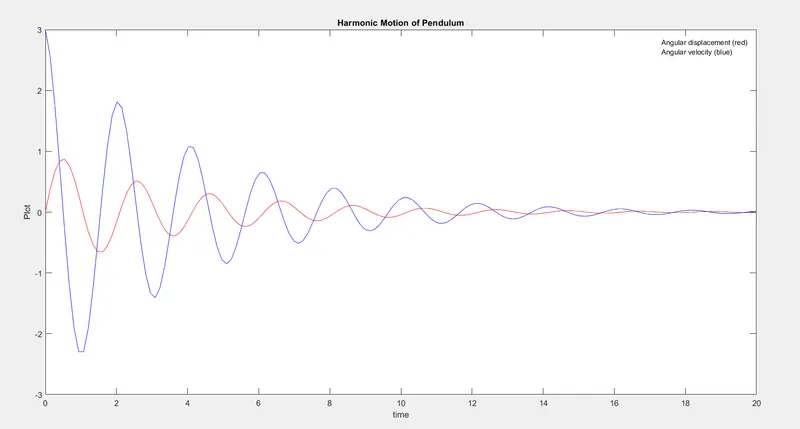
So as given in the code we can see displacement initial point is 0 and velocity initial point is 3.

So as the pendulum oscillation decreases the graph shows the same way.

Animation: