Week 3 - Solving second order ODEs

• Challenge Objective :

To write a program that solves the following ODE in Matlab\Octave that will simulate the pendulum motion to find angular dispacement and angular velocity of pendulum w.r.t to time.

where,

This ODE represents the equation of motion of a simple pendulum with damping.

• Introduction to ode45 solver :

MATLAB’s standard solver for ordinary differential equations (ODEs) is the function ode45. This function implements a Runge-Kutta method with a variable time step for efficient computation. ode45 is designed to handle the following general problem:

where t is the independent variable, x is a vector of dependent variables to be found and f(t, x) is a function of t and x. The mathematical problem is specified when the vector of functions on the right-hand side of above equation, f(t, x), is set and the initial conditions,x = x0 at time t0 are given.

In Engineering, ODE is used to describe the transient behavior of a system. A simple example is a pendulum,the way the pendulum moves depends on the Newtons second law. When this law is written down, we get a second order Ordinary Differential Equation that describes the position of the "ball" w.r.t time.

Similarly, there are hundreds of ODEs that describe key phenomena and if you have the ability to solve these equations then you will be able to simulate any of theses systems.in this challenge we will use ode45 solver to the the equation of motion of simple pendulum as shown below

How ode45 works:

The function ode45 takes 3 inputs. The 3 inputs are the function to be integrated, the time span and the initial conditions.The function would be one like shown in the above equation. The time span would be the integration limits. This can be provided as a vector of 2 values, the initial and final time or with a spacing using the linspace function. The solver will choose a step size that is most suitable for the solution to obtain the solution in the most optimal time as possible. The initial condition would be the value of the function at t=0s.

The function can be provided in the form of an anonymous function,

[t,results] = ode45(@(x) x^2, tspan,y0)

Here, we are saying that we don’t know the value of x and that x is an input to the anonymous function that we have defined here. This is equivalent to defining a function that takes the input of x and gives the output of x^2.

The function can also be defined as a separate function. This function must take at least 2 inputs, which should be t and y, apart from other arguments, where t would be the current time and y would be the value of the function at the previous time step.

Assuming we have a function ode, the function must be defined as, function [output] = ode(t,y,args).where args refer to any other arguments that the function may take.

This function must then be input to ode45 as [t,results] = ode45(@(t,y) ode(t,y,args), tspan, y0)

This is necessary to tell the function which arguments of the function are to be found by the solver.Thus, any ODE to be integrated by ode45 must be provided as a set of first order ODEs.

• Procedure for converting 2nd order into 1st orer ODE :

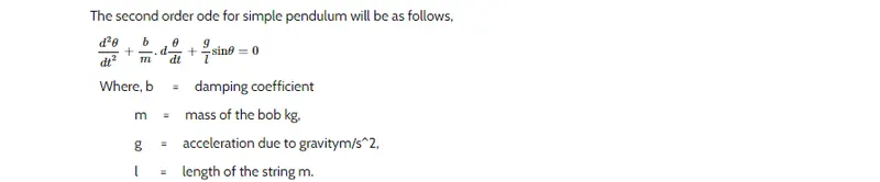
Now, we have been given 2nd order ODE of simple pendulum we will convert then into first order ODE.

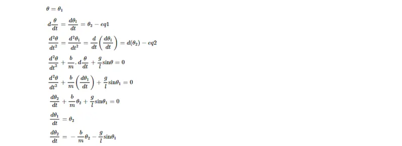
after converting into first order ODE we will be writing the two equations in vector form of matrix as shown below

`d/dt [(theta_1) ,(theta_2)]=[(theta_2),((-b/m)theta_2-(g/l)sintheta)]`

so the vector matrix above can be called as a solution vector since it contains two quantities.

• MAIN PROGRAM :

now we will solve it in programming in matlab :

first we will give inputs that we have recieved from the challenge which are

Damping coefficient	b = 0.05
Acceleration due to gravity (m/s2)	g = 9.81
Length of the pendulum (meter)	l = 1
Mass(kg)	m = 0.1

clear all
close all
clc

% Given inputs

b = 0.05;    %Damping coefficient
g = 9.81;    %Acceleration due to gravity (m/s2)
l = 1;       %Length of the pendulum (meter)
m = 0.1;     %mass (kg)

after giving inputs we will define the initial conditions,since we are solving ode .there are two first order ODE one is for displacement and another for velocity.

To solve the first ODE we need to provide intital conditions for displacement.here the initial dsplacement for pendulum is 0 and initial condition of velocity is 3 m/s which is written in matlab as theta_0 = [0 ; 3]

%Defining initial conditions where intial ang disp=0 & initial ang vel = 3
theta_0 = [0 ; 3];

%time points

t_span = linspace(0,20,250);

and the t_span is time array i.e., of 250 values that ranges from 0 to 20.here,tspan has two elements, [t0 tf], then the solver returns the solution evaluated at each internal integration step i.e., 250 steps within the interval.

Now we will form a syntax for creating function handle here so that we can call ODE function

here we are integrating the ODE system to obtain a solution.since we have already defined initial conditions theta_0 and time points t_span

%solveing ODE
[t,results] = ode45(@(t,theta) ode_func(t,theta,b,g,l,m),t_span,theta_0);

here ode45 main inputs are t and theta which are main dependent and independent variables of our ODE system.so we are saying that ODE is function of t and theta and then we are defining a function i.e., ode_func(t,theta,b,g,l,m) which is nothing but the seperate matlab program that we have written below.

FUNCTION PROGRAM :

function[dtheta_dt] = ode_func(t,theta,b,g,l,m)
  
 theta1 = theta(1)
 theta2 = theta(2)
 dtheta1_dt = theta2;
 dtheta2_dt = -(b/m)*theta2-(g/l)*sin(theta1);
 dtheta_dt = [dtheta1_dt;dtheta2_dt];
 
end

here we are passing t,theta,b,g,l,m which are input parameters into the function "ode_func".so " ode_func(t,theta,b,g,l,m) " is the ode function definition.inside of the function definition we are defining theta1 and theta2 by clubbing them into variable name " theta " which makes it as a solution array.so 1st value of theta gives theta(1) and 2nd value as theta(2).

so the first ode i.e., " dtheta1_dt = theta2 " and 2nd ode is " dtheta2_dt = -(b/m)*theta2-(g/l)*sin(theta1) " and then we combine them into an array called as " dtheta_dt = [dtheta1_dt;dtheta2_dt] " i.e., a column matrix since we have given ";" between them.

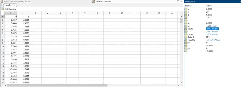
finally,the function " ode_func(t,theta,b,g,l,m) gives me integration time and results i.e., [t,results].since we are solving 2 ode's the result would be column vector with two columns in which 1st column refers to displacement and 2nd column refers to velocity as shown in the below picture from the workspace

then we will proceed with writing commands for plotting the results with label names specified on both the axis which is coded below.

% Plots
figure(1)
plot(t,results(:,1),'linewidth',1.5)
hold on
plot(t,results(:,2),'linewidth',1.5)
grid on
xlabel('time(s)')
ylabel('angular displacement & angular velocity')
legend('angular displacement','angular velocity')

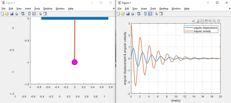
if we run the program it will give a plot :

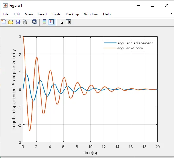
In order to animate the pendulum we will make use of for loop with displacemt values in results vector as input

for i = 1 : length(results(:,1)) where i value varies from 1 to length of results in first column i.e., angular displacement so that we can able to see the movemnt of pendulum.

the first end of the pendulum will be fixed to a point so we will take the values x0 = 0 and y0 = 0 and x1 y1 depends on the inputs form the results which varies w.r.t angular displacement where, x1 = length of string * sind(theta) is coordinate value at theta1 in x axis and y1 = length of string * cosd(theta) is coordinate value at theta1 in y axis .

After specifying the both end cordinate values we will be able to plot the animation using plot command for both angular displacement and angular velocity with hold command.

% Creating the animation of pendulum by plotting coordinates
ct = 1;
for i = 1 : length(results(:,1));
 x0 = 0;
 y0 = 0;
 
 x1 = l*sin(results(i,1));       % coordinate value at theta1 in x axis      
 y1 = -(l*cos(results(i,1)));      % coordinate value at theta1 in y axis 
 
 % plots
 figure(3)
 plot([-0.75 0.75],[0 0],'color','#0072BD' ,'linewidth',10 );
 axis([-1 1 -1.5 0.10])
 hold on
 plot([x0,x1],[y0,y1],'linewidth',3,'color','#D95319');
 plot(x1,y1,'o','markersize', 20, 'markerfacecolor', 'm','color','k');
 pause(0.03)
 hold off
M(ct) = getframe(gcf);
ct = ct+1;

end

we make use of movie command that creates a movie which is a video of a simple pendulum in avi format that we have specified already by attaching all the plots together.

movie(M)
videofile = VideoWriter('pendulum_ode_by_saibhaskar.avi','Uncompressed AVI');
open(videofile)
writeVideo(videofile,M)
close(videofile)

Error 1 : Invalid expression. When calling a function -

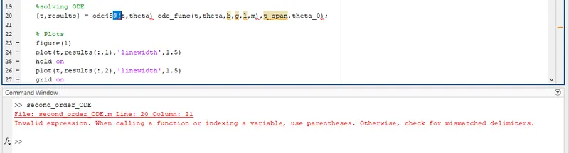
sol : Here i havent specified the paranthesis after the ode45@ which gives an invalid expression and makes the code useless so make sure to check for all symbols and expressions are included in correct way. so here we have to give open bracket to complete the line of code so that it will take it as a valid function i.e, [t,results] = ode45(@(t,theta) ode_func(t,theta,b,g,l,m),t_span,theta_0);

Error 2 :

Error in ode_func (line 3)
theta1 = theta(1) ,not enough input arguments

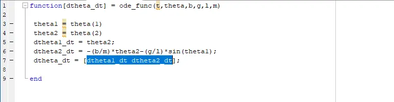
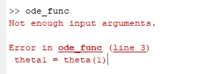
sol : so actually the error is solved by seperating dtheta1_dt dtheta2_dt in line7 by ";" as ahown below so that it will create two rows in vector matrix which makes theta = theta(1) valid statement.

RESULT :

clear all
close all
clc

% Given inputs

b = 0.05;    %Damping coefficient
g = 9.81;    %Acceleration due to gravity (m/s2)
l = 1;       %Length of the pendulum (meter)
m = 0.1;     %mass (kg)

%Defining initial conditions ang disp=0 &  ang vel = 3
theta_0 = [0 ; 3];

%time points

t_span = linspace(0,20,250);

%solving ODE
[t,results] = ode45(@(t,theta) ode_func(t,theta,b,g,l,m),t_span,theta_0);

% Plots
figure(1)
plot(t,results(:,1),'linewidth',1.5)
hold on
plot(t,results(:,2),'linewidth',1.5)
grid on
xlabel('time(s)')
ylabel('angular displacement & angular velocity')
legend('angular displacement','angular velocity')


% Creating the animation of pendulum by plotting coordinates
ct = 1;
for i = 1 : length(results(:,1));
 x0 = 0;
 y0 = 0;
 
 x1 = l*sin(results(i,1));       % coordinate value at theta1 in x axis      
 y1 = -(l*cos(results(i,1)));      % coordinate value at theta1 in y axis 
 
 % plots
 figure(3)
 plot([-0.75 0.75],[0 0],'color','#0072BD' ,'linewidth',10 );
 axis([-1 1 -1.5 0.10])
 hold on
 plot([x0,x1],[y0,y1],'linewidth',3,'color','#D95319');
 plot(x1,y1,'o','markersize', 20, 'markerfacecolor', 'm','color','k');
 pause(0.03)
 hold off
M(ct) = getframe(gcf);
ct = ct+1;

end

movie(M)
videofile = VideoWriter('pendulum_ode_by_saibhaskar.avi','Uncompressed AVI');
open(videofile)
writeVideo(videofile,M)
close(videofile)

function[dtheta_dt] = ode_func(t,theta,b,g,l,m)
  
 theta1 = theta(1)
 theta2 = theta(2)
 dtheta1_dt = theta2;
 dtheta2_dt = -(b/m)*theta2-(g/l)*sin(theta1);
 dtheta_dt = [dtheta1_dt;dtheta2_dt];
 
end