Week 3 - Solving second order ODEs

PROBLEM STATEMENT: To create an animation of the pendulum oscillation by using the solution obtained from solving the ordinary differential equation(ODE) for the phenomenon using python programming language.

OBJECTIVE: To create an accurate animation of the pendulum oscillation after solving the ODE governing the phenomenon using python.

SOLUITION AND CODE: The ordinary differential equations (ODE) can be solved in python using the scipy.integrate module. Specifically odeint.

The code for solving is as follows.

import math
from scipy.integrate import odeint
import numpy as np
import matplotlib.pyplot as plt

#allocating values for the various constants
L=1 #metre

m=1 #kg

b=0.05

g=9.81 #m/s2

#ode describing model function
def model(theta , t , b , g , l , m):
	theta1=theta[0]
	theta2=theta[1]
	dtheta1_dt = theta2
	dtheta2_dt = -(b/m)*theta2 - (g/L)*math.sin(theta1)
	dtheta_dt = [dtheta1_dt,dtheta2_dt]
	return dtheta_dt

#creating an array of time steps for integration
t = np.linspace(0,20,300)

#initial conditions t=0
theta_initial = [0 , 3]

#solve ODE
theta = odeint(model , theta_initial , t, args=(b,g,L,m))

#plotting
plt.plot(t,theta[:,0] , 'b-',label=r'$\frac{d\theta_1}{dt}=\theta_2$')
plt.plot(t,theta[:,1] , 'r--',label=r'$\frac{d\theta_2}{dt}=-\frac{b}{m}\theta_2-\frac{g}{l}sin\theta_1$')
plt.xlabel('plot')
plt.ylabel('time')
plt.legend(loc='best')
plt.show()

For solving the ODE , we first define the model describing function. This function is just the python version of the mathematical differential representation.Also the various constants involved are defined accordingly.

Now initial conditions i.e initial angular velocity and angular acceleration is defined in an array.

The variable 'theta' contains lists of the solutions. That is the angular velocity for each finite time and angular acceleration for each finite time.

Now plot is made with suitable labels and legends using the matplotlib.pyplot module.

RESULTS AND OBSERVATION:

The plot is follows.

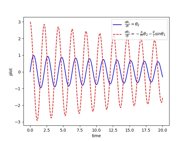
We can observe the curve's amptitude draining out solwly as time proceeds. This is because of the non zero damping coefficient.

Thus the ODE for the simple pendulum oscillation phenomenon has been successfully solved and plot for its solution is successfully made.