Week 3 - Pitot tube
SIMULATION OF PITOT STATIC TUBE:
1 INTRODUCTION:
Static pressure: It is a measure of the purely random motion of molecules in the gas. It is the pressure along the local flow velocity of the gas.
Total pressure / Stagnation pressure: It is the pressure that the flow achieves when the velocity is reduced to zero.
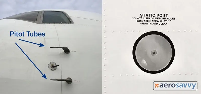
It is possible to combine both the measurement of total and static pressure in one instrument called the Pitot-Static tube. It is used to measure the speed of the airplane, it should be located on the air-plane in a position where it is essentially immersed in the freestream flow, away from any major influence of the local flow field around the airplane itself. The term Indicated Air Speed is used for the measurement made with an actual air speed indicator. Owing to the instrument error, IAS will normally differ from EAS (Equivalent Air Speed). Therefore, IAS is the uncorrected reading shown by an actual air-speed indicator. EAS is the uncorrected reading that would be shown by a hypothetical error-free air-speed indicator. True Air Speed (TAS) is the actual speed of the aircraft relative to the air. In Modern day aircrafts, the conversion from IAS to TAS is done electronically.
However, the main use of Pitot tubes is to measure the velocity of solid bodies moving through fluids, such as the velocity of ships and of low speed aircraft. In these cases, the tube is connected to a Bourdon pressure gauge which can be calibrated to read velocity directly. A development of the Pitot tube, a pitometer, tests the flow of water in water mains and detects leakages.
2 THEORY OF PITOT-STATIC TUBE:
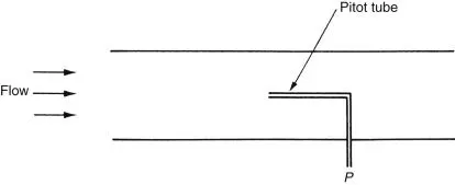
The Pitot-static tube is mainly used for making temporary measurements of flow, although it is also used in some instances for permanent flow monitoring. It measures the local velocity of flow at a particular point within a pipe rather than the average flow velocity as measured by other types of flowmeter. This may be useful where there is a requirement to measure local flow rates across the cross section of a pipe in the case of non-uniform flow. Multiple pitot tubes are normally used to do this. The instrument depends on the principle that a tube placed with its open end in a stream of fluid. Will bring to rest that part of the fluid that impinges on it, and the loss of kinetic energy will be converted to a measureable increase in pressure inside the tube. This pressure as well as the static pressure of the undisturbed free stream of flow is measured.
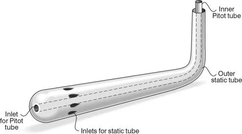
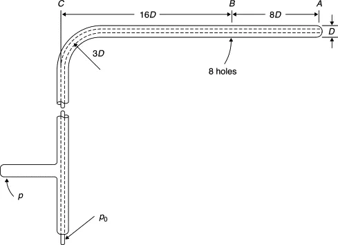
The Pitot-static tube consists of two concentric tubes, the central one with an open end pointing upstream of the fluid flow and the other closed at the end but with small holes drilled at right angles to the direction of flow. The central tube pressure is equal to the static pressure plus the ‘velocity pressure’, whereas the outer tube pressure is the static pressure only.
Total pressure = Static pressure + Dynamic pressure
Pressure = `1/2 rho v^2`
V=`sqrt((2(Pt-Ps))/rho)`
From the above relation, Velocity can be found from pressure values of static and total pressure. The computational velocity value is found from the computational result pressure values, which is compared to the numerical velocity value and hence the efficiency of the solver can be assessed.
3 COMPUTATIONAL SETUP:
3.1 Setting the geometry and meshing
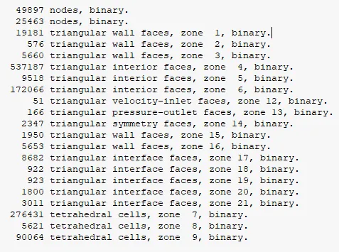
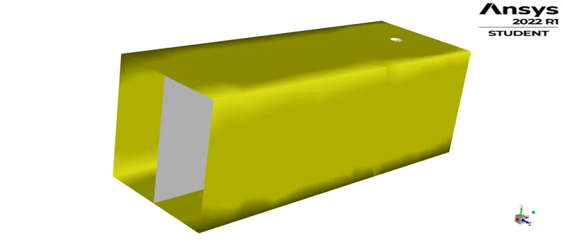
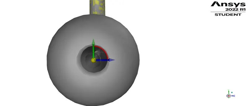
The geometry consists of an enclosure with a pitot-static tube. The inlets and outlets are named and the model is meshed conveniently.
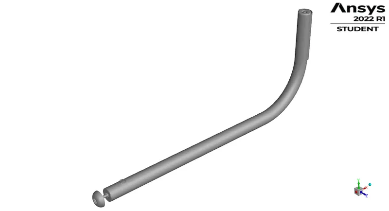
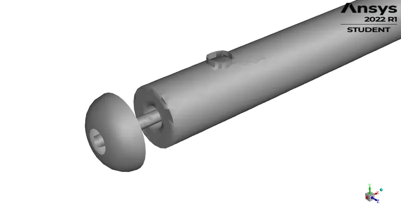
A center XY plane and two monitoring points are made to define the variables. Two points one at the mouth of the tube to measure the total pressure and one at the static port opening near the wall is made for measuring the static pressure.

3.2 Setting the Fluent solver
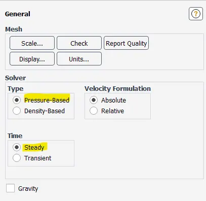
3.2.1 General solver conditions
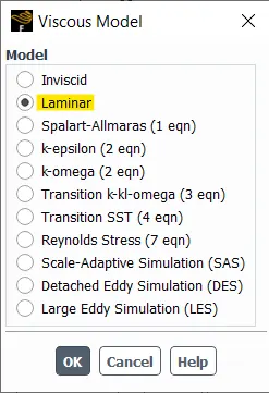
A pressure-based laminar solver is used for the computation.
3.2.2 Boundary conditions
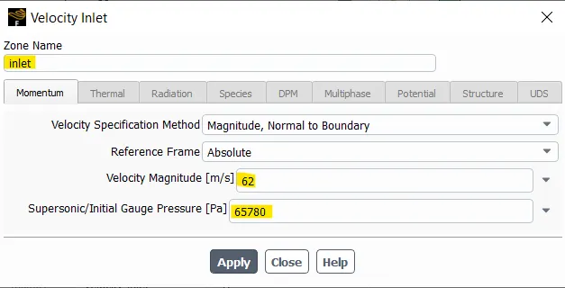
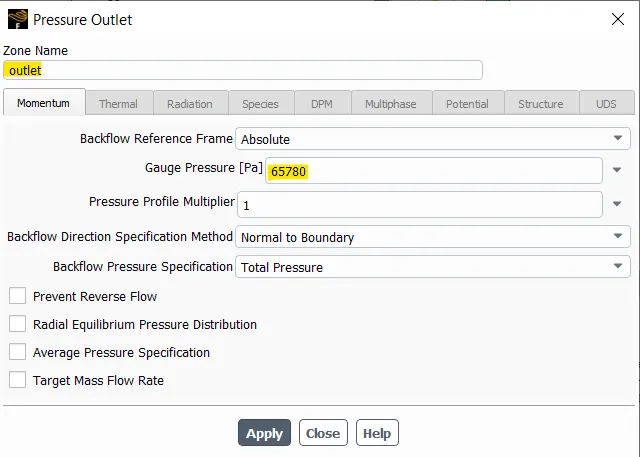
A velocity inlet and pressure inlet is defined using the given numerical values as the gauge pressure.
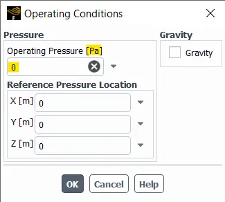
The Operating pressure is set at 0pa.
3.2.3 Material properties
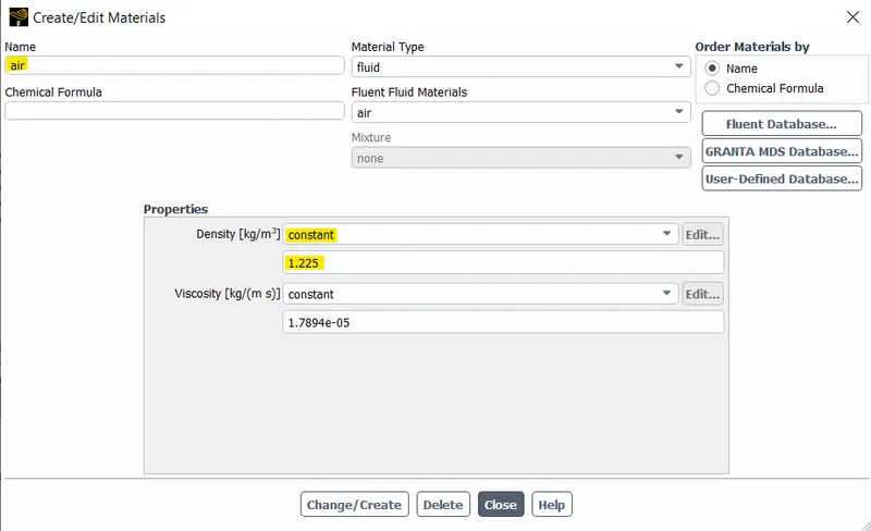
The air with constant density used by default.
3.2.4 Variable and contour definitions for post-processing
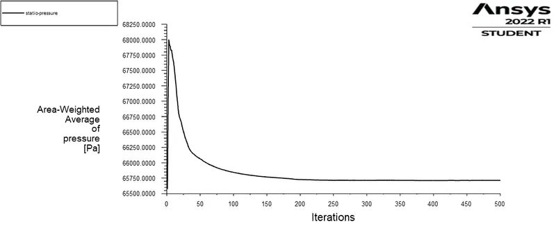
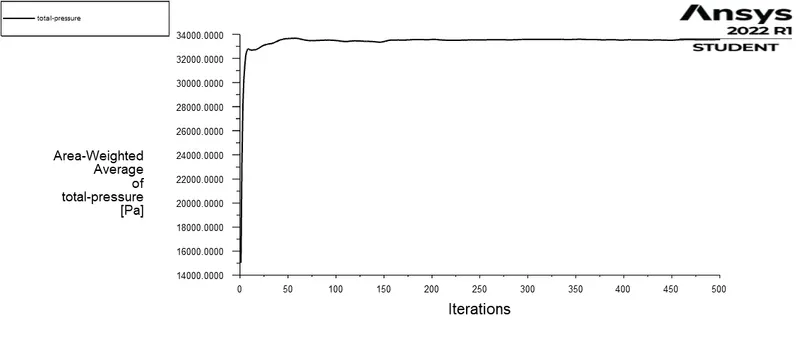
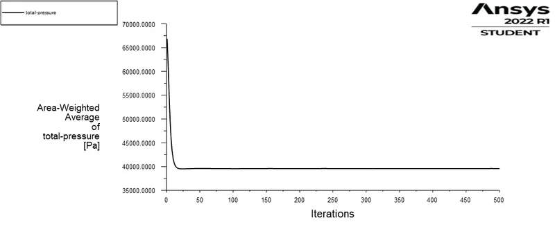
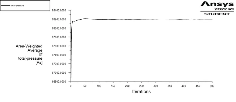
Static pressure graph at the static point and total pressure graph at the total pressure point is defined.
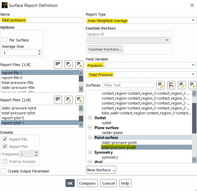

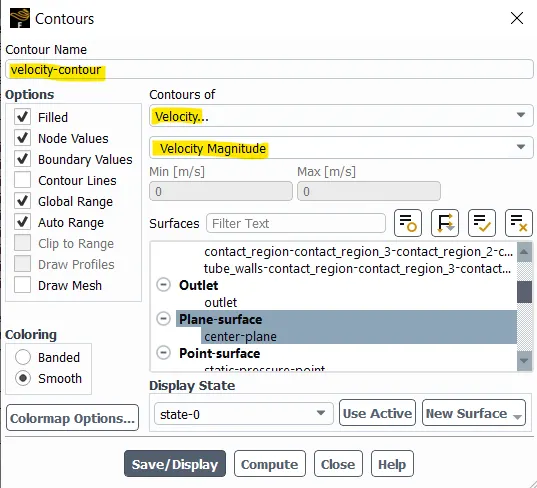
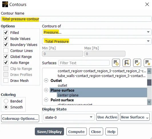
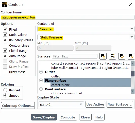
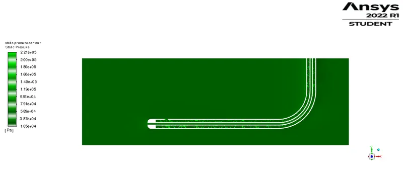
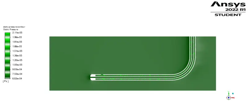
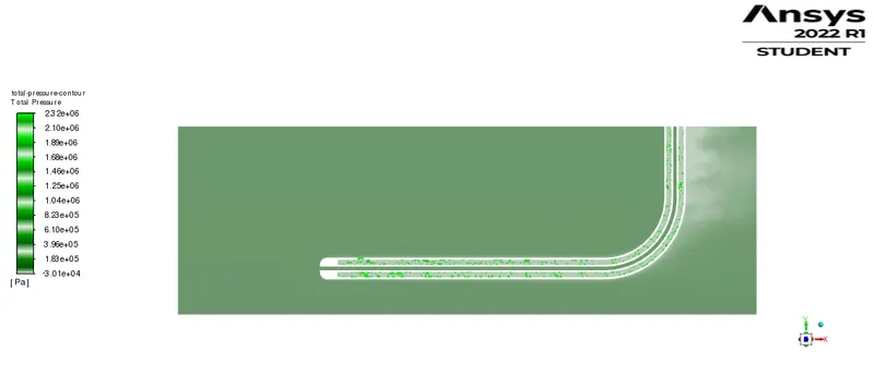
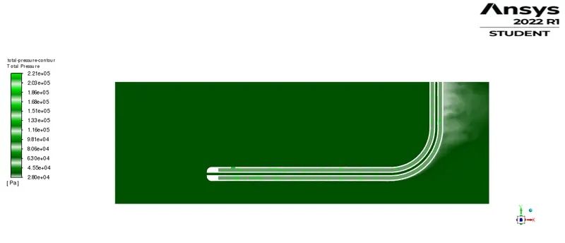
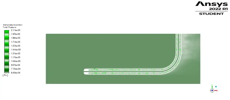
Contours for velocity, static pressure and total pressure are defined at the center plane created.
3.3 Run Cases
3 cases with different velocity and gauge pressure is run for 500 iterations after a hybrid initialization.
|
Case 1: |
Case 2: |
Case 3: |
|
Velocity = 240m/s Gauge pressure = -2817 pa |
Velocity = 100m/s Gauge pressure = 33287 pa |
Velocity = 62m/s
Gauge pressure = 65780 pa |
4 COMPUTATIONAL RESULTS:
4.1 Result data:
|
Case 1: |
Case 2: |
Case 3: |
|
| Total pressure |
33538 pa |
39590.55 pa |
68199.465 pa |
| Static pressure |
-3751 pa |
33223.726 pa |
65714.526 pa |
4.2 Contours:
| Case 1: 240m/s, -2817pa | Case 2: 100m/s, 33287pa | Case 3: 62m/s, 65780pa |
|
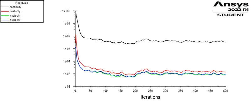
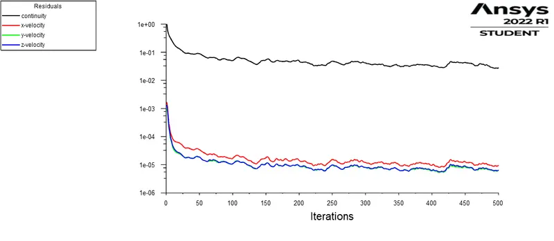
Residuals plot:
|
Residuals plot:
|
Residuals plot:
|
|
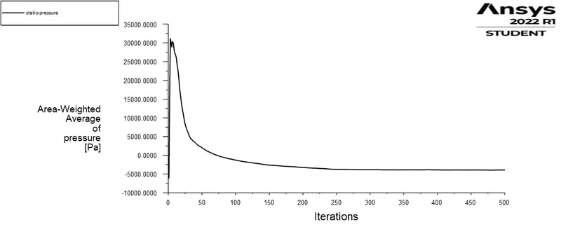
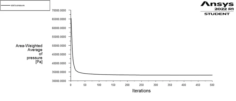
Static pressure plot:
|
Static pressure plot:
|
Static pressure plot:
|
|
Total pressure plot:
|
Total pressure plot:
|
Total pressure plot:
|
|
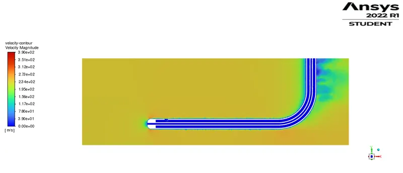
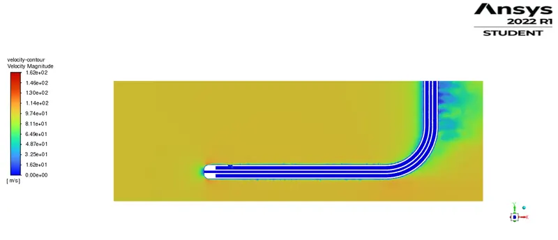
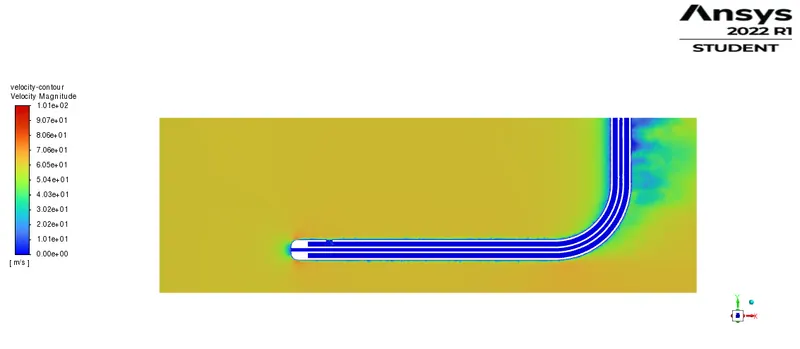
Velocity contour:
|
Velocity contour:
|
Velocity contour:
|
|
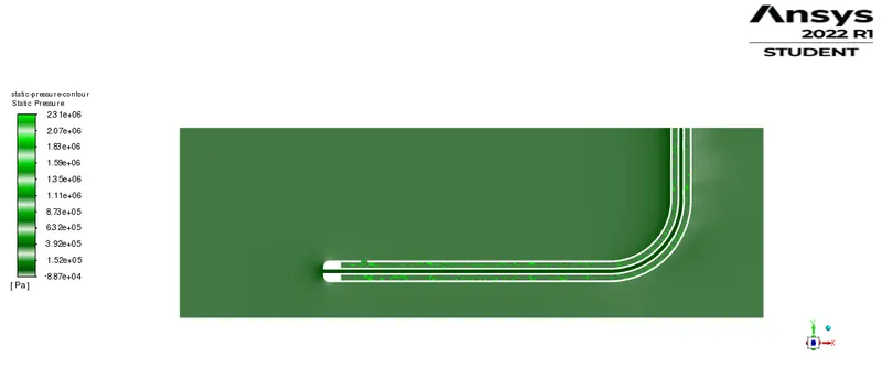
Static pressure contour:
|
Static pressure contour:
|
Static pressure contour:
|
|
Total pressure contour:
|
Total pressure contour:
|
Total pressure contour:
|
5 INFERENCE:
| Case 1: | Case 2: | Case 3: | ||
| Numerical value | Velocity | 240 m/s | 100 m/s | 62 m/s |
| Numerical value | Gauge pressure | -2817 pa | 33287 pa | 65780 pa |
| Computational result | Total pressure | 33538.78 pa | 39590.55 pa | 68199.465 pa |
| Computational result | Static pressure | -3751 pa | 33223.726 pa | 65714.526 pa |
| Computational result | Velocity | 246.74 m/s | 101.95 m/s | 63.69 m/s |
| Solver efficiency | Error % | 2.8% | 1.95% | 2.72% |
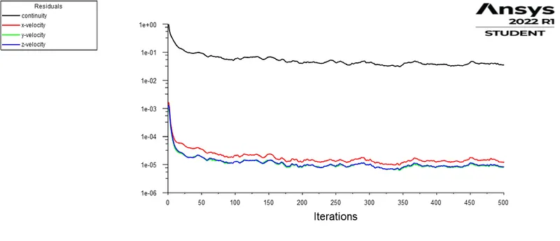
From the above results, it is evident that the efficiency of the solver, ANSYS Fluent is around 98%. This implies that the solver is conveniently suitable for similar kind of applications. The contours also depict that the velocity inside the tubes are zero, and hence the physics behind the pitot-tube. It is also seen from the pressure contours, that there a certain high gradient of pressure inside the tubes, which may be due to the momentum buildup of the fluid flow. To avoid this in the result, the simulation is run for a certain period of time and the value is taken after the convergence of the solution. This can be seen from the pressure plots, where the result value is the average value from the straight line.
Regarding the solver environment, the operating pressure is maintained at 0Pa, which gives the absolute value for pressure. The boundary conditions are set at walls, and symmetry, which gives an accurate measurement of the computational domain, which adds up to the solver efficiency. Clearly, three cases of different pressure values with a negative pressure is also taken to get precise. The flow separation in the backside of the elbow of the pitot-tube has a dispersion seen in pressure tube, which is result of the flow being obstructed by the tube inside the domain. These are not seen near the walls, probably due to the boundary conditions. In real-life practical approach, this is achieved by placing the pitot-tube farther away from the fuselage of the aircraft, where the effect of turbulence and boundary layer on the pitot tube due to the fuselage is very minimal or zero. The small pressure gradients inside the tube is also avoided by having a design of perfect length to the diameter ratio, which is calculated from experiments and simulations, depicted in the theory section above.
6 CONCLUSION:
Thus the pitot-static tube's function can be validated using computation values, which are further compared with the experimental data for its design. The efficiency of the solver is performing these computations is also validated which forms the base for the selection of methods among experimental, numerical, and analytical methods. In some instances, all these methods are needed to design a component before using it in real-life applications. Studies like these portray the prediction level accuracy of the methods to be able to employ them in analyzing a component.
7 REFERENCE:
Fundamentals of Aerodynamics, Sixth edition, John D. Anderson,Jr.
William Gracey, ... Tony Whitmore, in Encyclopedia of Physical Science and Technology (Third Edition), 2003