Week 3 - Pitot tube

Aim --> Pitot tube simulation using Ansys fluent.

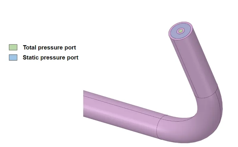
1. A pitot static tube geometry is attached below.

a.You are required to do a literature review of pitot-static tube. Also establish a relationship between Total (stagnation) pressure and static pressure.

b.You are required to create surfaces and fill it separately for Total pressure port and static pressure port as shown below.

Introduction

A pitot tube is a flow measuring device used to measure fluid velocity. It is widely used to determine the airspeed of an aircraft, water speed of a boat, and to measure liquid, air and gas flow velocities in certain industrial applications.

The basic pitot tube consists of a tube pointing directly into the fluid flow. As this tube contains fluid, a pressure can be measured; the moving fluid is brought to rest (stagnates) as there is no outlet to allow flow to continue. This pressure is the stagnation pressure of the fluid, also known as the total pressure or (particularly in aviation) the pitot pressure.

The dynamic pressure, then, is the difference between the stagnation pressure and the static pressure. The dynamic pressure is then determined using a diaphragm inside an enclosed container. If the air on one side of the diaphragm is at the static pressure, and the other at the stagnation pressure, then the deflection of the diaphragm is proportional to the dynamic pressure.

In aircraft, the static pressure is generally measured using the static ports on the side of the fuselage. The dynamic pressure measured can be used to determine the indicated airspeed of the aircraft.

Stagnation pressure = static pressure + dynamic pressure

Using this relation we can compute for velocity once we know the static and stagnation pressure with the following equation.

• we employ pressure based steady-state solver.
• air is the fluid. density = 0.863 Kg/m3 and viscosity = 1.678e-5 m2/s
• Operating pressure is 0 Pa.
• we perform hybrid initialization.(we can also opt for standard initialization followed by FMG Initialization.)
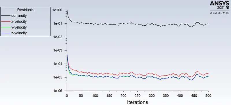
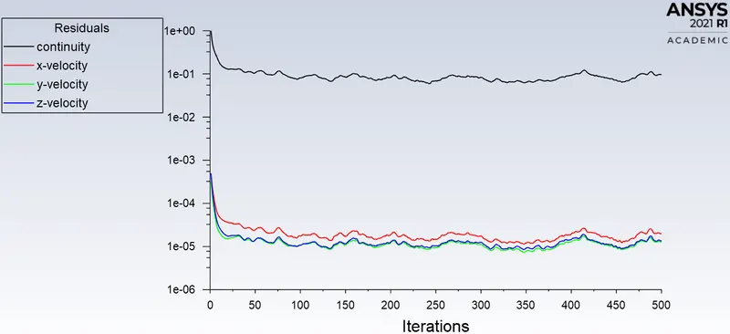
• 500 Iterations.

Results

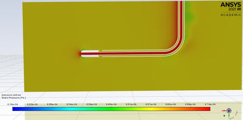
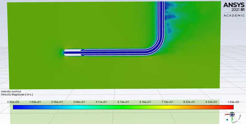
Case I --> v = 62 m/s, Gauge Pressure 65780 Pa

Residual

Pressure plot

Velocity contour

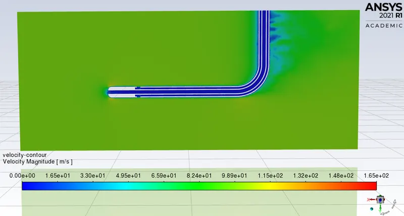
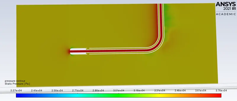
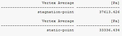
Case II --> v=100 m/s Gauge Pressure 33287 Pa

Residual

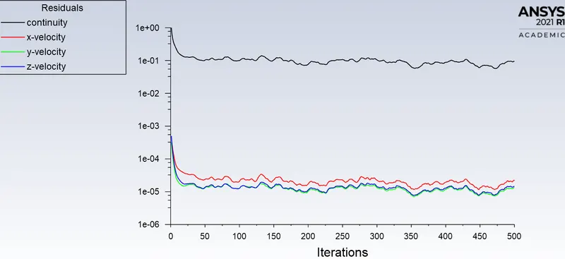
Velocity contour

pressure contour

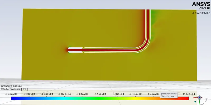
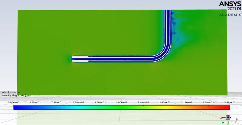
Case III --> v=240 m/s Gauge Pressure -2817 Pa

Residual

Pressure contour

Velocity contour

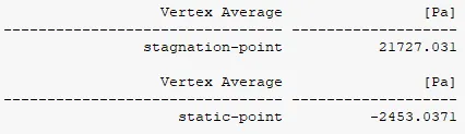
Given velocity	62	100	240
stagnation pressure	67442.414	37613.426	21727.031
static pressure	65791.172	33336.434	-2453.0371
calculated velocity	61.8607189	99.55	236.7218
% error	0.224	0.45	1.365

Conclusion

The results were obtained from Ansys Fluent and validated by using the bernoulli's principle.