Week 3: Flow over a backward facing step

Aim:

• To simulate the Backward step flow for three different mesh grid sizes by using convergentscience and paraview.
• To show various velocity and pressure contours for the different mesh.
• To show the various plot of velocity, pressure, mass flow rate and total cell count fordifferent mesh grids.
• To steady the turbulent flow characteristics in Backward step flow

Introduction:

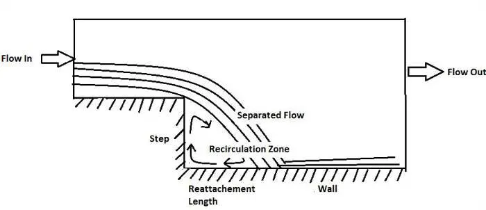
Fully developed flow enters the domain from left. When the flow reaches the step, becauseof expansion of flow channel, pressure gradient exists, it detaches and a recirculation zoneis formed. A turbulent boundary layer encounters a sudden back step, causing flowseparation. Later the flow eventually reattaches to the bottom wall.

Backward-Facing Step (BFS) flow is one representative model for separation flows, whichcan be widely seen in aerodynamic flows (airfoil, spoiler, high attack angle process),engine flows, condensers, vehicles (cars, boat), heat transfer systems, and even the flowaround buildings, etc. The flow separation after a simple stage will introduce separationbubble formation, evolution and re-attachment process, which is dependent on theBackward Facing Step geometric design, the inlet and outlet conditions, turbulent intensity,as well as heat transfer conditions. It is shown that the step size (duct expansion ratio) willdefine the basic re-circulation and re-attachment process.

It is a basic model involving the most important feature of a separated flow –a free shearflow separation, vortex generation and reattachment.

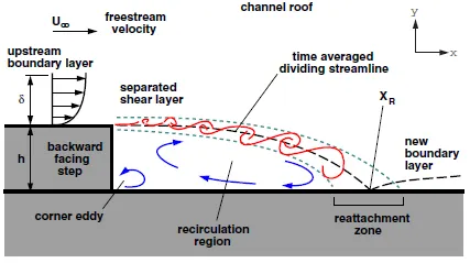
A backward step flow includes an inflow of uniform velocity,laminar or turbulent from achannel to a step on the either sides with a step height of h .The flow fluid is divided intofour regions namely separated Shear layer ,the recirculation region under the shearlayer,the reattachment region, and the recovered boundary layer.

Flow with separation and reattachment has long been a subject of fundamental fluiddynamics research. The presence of a separated flow, together with a reattaching flow,gives rise to increased unsteadiness, pressure fluctuations, structure vibrations and noise,as it also exhibits an unsteady structure with a large scale vortex in the separated group(RNG) k-ε model to account for turbulent viscosity.Turbulent flows occur in a variety of industrial problems. A flow is termed as turbulent whenthe inertial forces of the fluid are greater than the viscous forces resulting in chaoticfluctuations in the flow.

Importance of Backward Facing Step Problem

Separation and reattachment of turbulent flows occur in many practical engineeringapplications. It is seen both in internal flow systems such as diffusers, combustors andchannels with sudden expansions, and in external flows like flow around airfoil and building.In these situations, the flow experiences an adverse pressure gradient, which causes theboundary layer to separate from the solid surface. The flow subsequently reattachesdownstream forming a recirculation bubble. The presence of a separated flow, togetherwith a reattaching flow, gives rise to increased unsteadiness, pressure fluctuations whichmay lead to structure vibrations and noise.

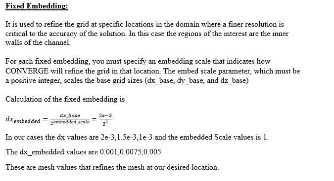
Procedure for Generation of Geometry:

We have to create the geometry of the Backward step flow in the Converge by using theCommands provided in the geometry box.The dimensions of the geometry is shown in thebelow image.

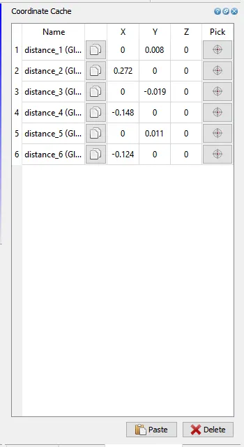
Go to the create geometry and by using vertices method enter the Co-Ordinates of thevertices and then join them by using the 3 vertices triangle method and then copy thegeometry by using the angle method and copy the geometry at the distance of -0.02meters in the direction of Z-axis then by using the loft command we can complete the 3dgeometry of the Backward step.The below figure shows the geometry.

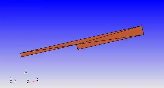
Now enables the normal/Vectors of the geometry and transform the normal in one direction.

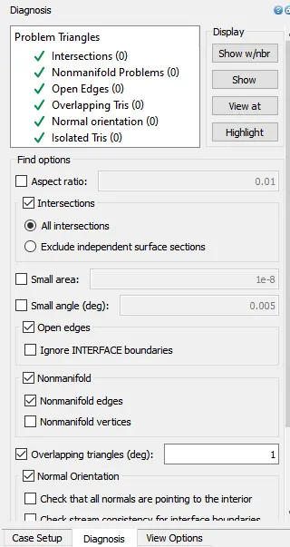
Now check for the errors in the Diagonsis Dock.Check for the errors in Intersections, Openedges,Over lapping triangles and for isolated triangles if there was no errors means we canforward for the case setup.

case setup for simulation:

• In the Run Parameter: Solver we used is Steady state and the simulation mode = Fullhydrodynamic in the mic state we enable the Solver Momentum, Solve Species and Steadystate Monitor.
• In the Steady State Monitor, we keep the minimum number of Cycles to be execute forSteady State solver is 15000 and we add the monitor variables of Mass flow rate andaverage velocity
• In Simulation time Parameters we set the values for start time as 0 cycles and end time15000 cycles and the initial and Minimum time setup for 1e-9 and remaining values are putto default
• In the Solver Parameters, the Navier stock equation should be Pressure based solver andremaining should be default.
• The number of cycles for the 2e-4 mesh, 1.5e-4 and 1.2e-4 is 15000 in order to converge thesolution.

Initialization and Boundary condition:

• In the initialization region change the name of the Region as a volumetric region and thevalues assigned for the temperature and pressure is 300k and 101325.0 Pascal and add the species O2 and N2 with the mole fraction of 0.23 and 0.77.
• The pressure at the inlet is 110325 Pascal and the temperature should be 300 k and theboundary type is INFLOW
• The pressure at the outlet is 101325 Pascal and the temperature should be 300 k and theboundary type is OUTFLOW.
• For the Top and Bottom boundary should be the wall type with a Law of wall boundarycondition and temperature should be 300k.
• The front_2d and back_2d and the boundary type is 2D wall.
• The number of cycles for the 2e-4 mesh, 1.5e-4 and 1.2e-4 is 15000 in order to converge the solution.

Grid Control:

Results:

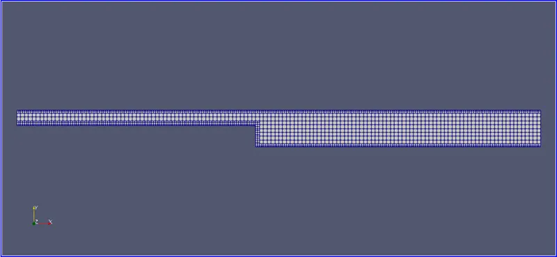
Case-I: dx = dy = dz =2e-3m Mesh size

• Mesh Profile:

• Velocity contours:

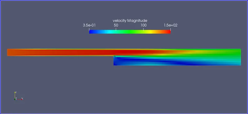
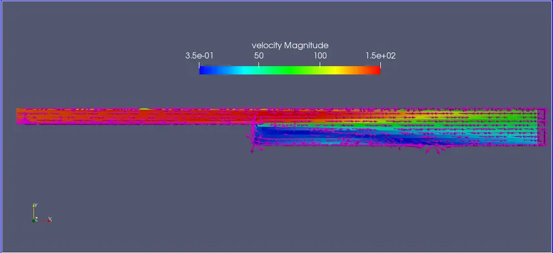
In the velocity counturs with the vectors the velocity after the step is recirculating becauseof the separation in the flow and form the boundary layer with the shear zone and atdistance forming a vortex which is the region for recirculating the flow.

• Velocity animation:

• Velocity plot

• Pressure contours

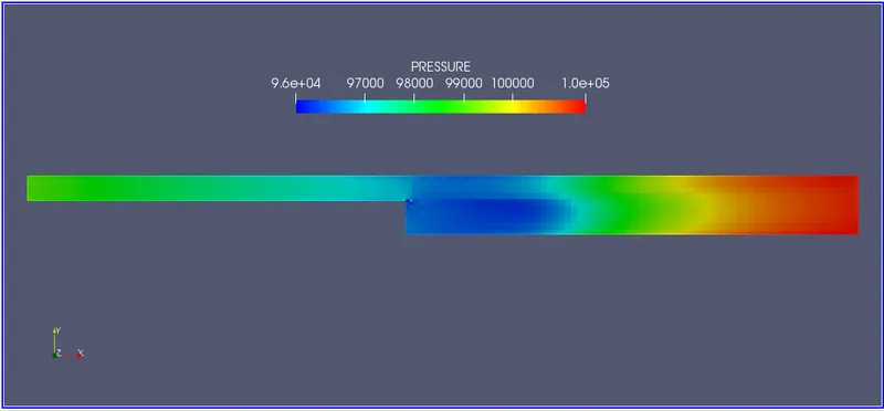
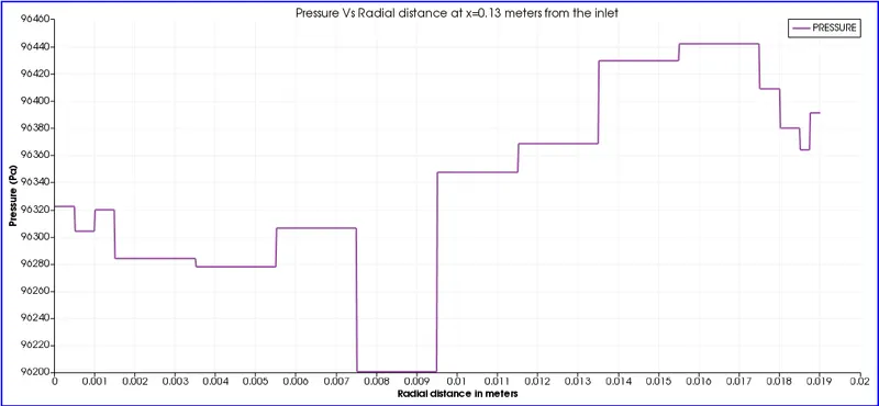
Initially the pressure is high at the inlet and it goes on increasing utill it reaches the stepregion and after that the pressure gradually changed it becomes lower in the step regiondue to the turbulence,the flow experiences an adverse pressure gradient, which causes theboundary layer to separate from the solid surfaces and after that there is a tremendousgrowth in the pressure untill it reaches the outlet and attains the maximum pressure.

• Pressure animations

• Pressure plot

• Mass flow rate

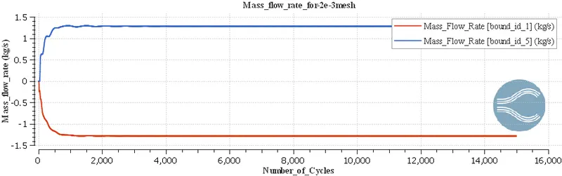
The mass flow rate is same for both inlets and outlets they are liked mirror image.Theconvergence is achieved after the 3500 cycles and value for the mass flow rate is 1.35kg/sec.

• Total Pressure at the inlet and outlet

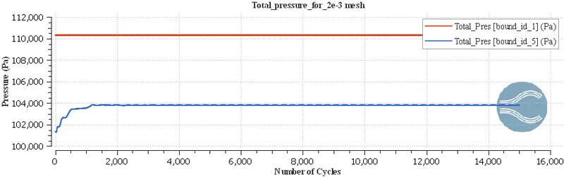
The pressure is constant at the inlet and the pressure at the outlet is gradually increasedfrom the starting cycles and achieved the convergence after the 2000 cycles and reaminsthe same value throughout the simulation.

• Average velocity at the inlet and outlet

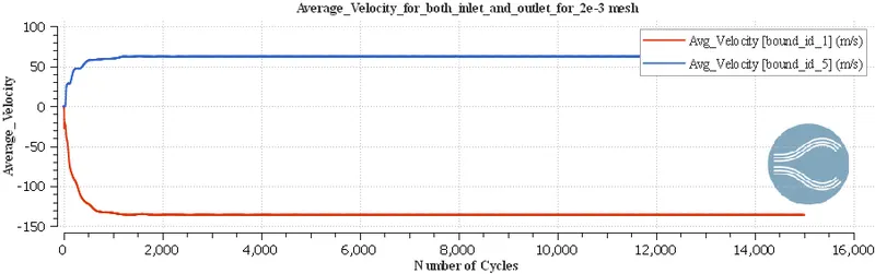
The Velocity at the inlet is -140 m/sec and the velocity at outlet is 60 m/sec.The velocity ishigh in the inlet and low at the outlet because of the increased cross sectional area for theoutlet when compared with the cross sectional area of the inlet.

• Total cell counts

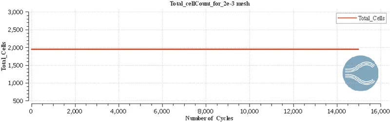
The total number of cells is around 1960 cells.The number of cells are low and the outputsof all graphs and plots are not smooth.

Case-II:

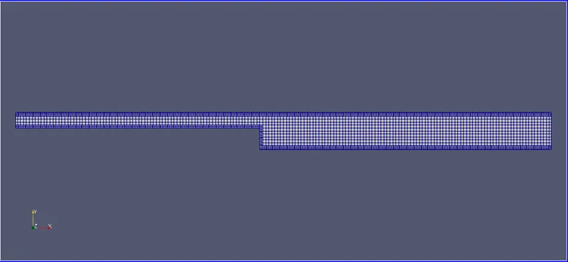
dx = dy = dz =1.2e-3m Mesh size

• Mesh Profile

• Velocity contour

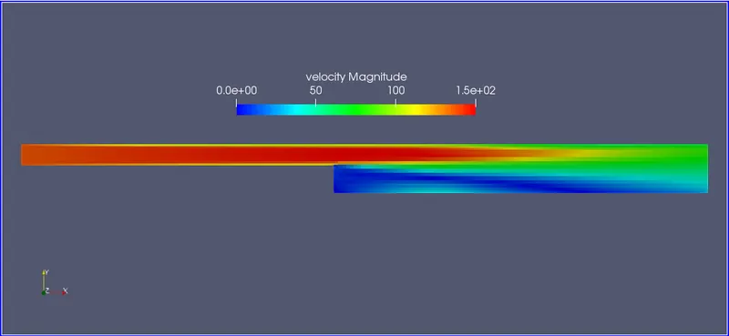
From the above image approximately of 60 m/sec due to the increased in the geometry and at the step thevelocity is very low due to the divergent nozzle and the flow is turbulent so the pressuredroping takes places so that the velocity starts decreasing from this point only.

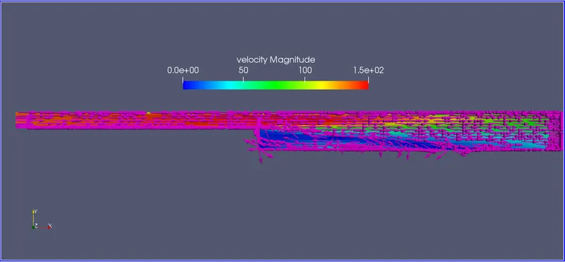
In the velocity counturs with the vectors the velocity after the step is recirculating becauseof the separation in the flow and form the boundary layer with the shear zone and atdistance forming a vortex which is the region for recirculating the flow.

• Velocity animation

• Velocity plot

• Pressure contour

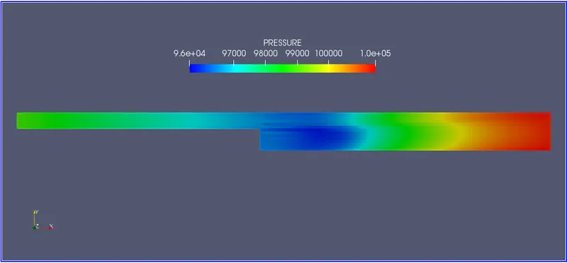
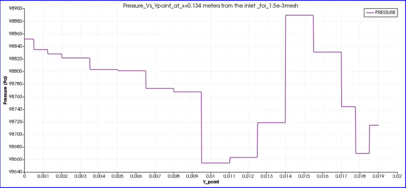
Initially the pressure is high at the inlet and it goes on increasing utill it reaches the stepregion and after that the pressure gradually changed it becomes lower in the step regiondue to the turbulence,the flow experiences an adverse pressure gradient, which causes theboundary layer to separate from the solid surfaces and after that there is a tremendousgrowth in the pressure untill it reaches the outlet and attains the maximum pressure.

• Pressure animation

• Pressure plot

• Mass flow rate

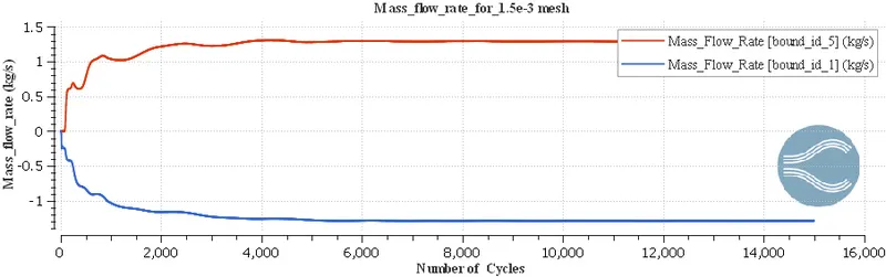
The mass flow rate is same for both inlets and outlets they are liked mirror image.Theconvergence is achieved after the 6000 cycles and value for the mass flow rate is 1.35kg/sec.

• Total pressure at the inlet and outlet

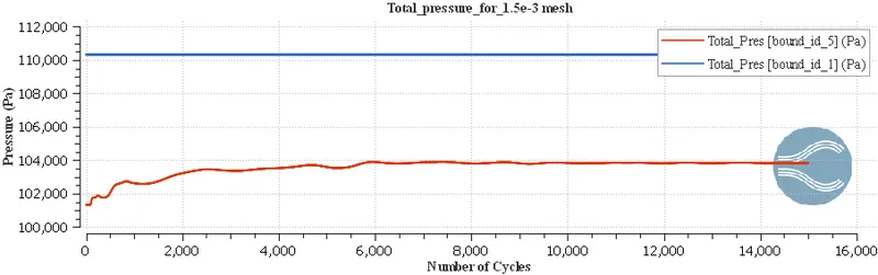
The pressure is constant at the inlet and the pressure at the outlet is gradually increasedfrom the starting cycles and achieved the convergence after the 6000 cycles and reaminsthe same value throughout the simulation.

• Average velocity at the inlet and outlet

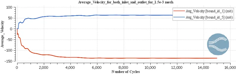
The Velocity at the inlet is -140 m/sec and the velocity at outlet is 60 m/sec.The velocity ishigh in the inlet and low at the outlet because of the increased cross sectional area for theoutlet when compared with the cross sectional area of the inlet.

• Total cell counts

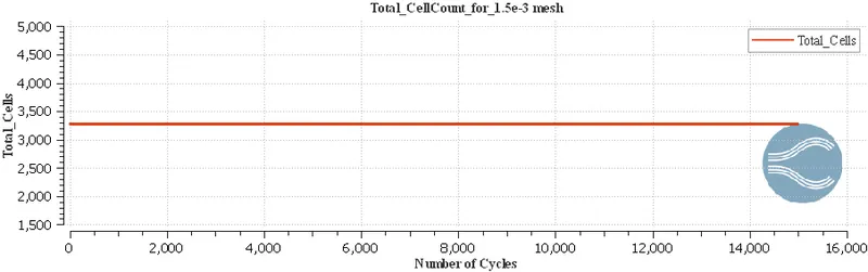
The total number of cells is around 3300 cells.The number of cells are increased beacuseof the refinement of mesh and the outputs of all graphs and plots are little bit smoother.

Case-III:

dx = dy = dz =1e-3m Mesh size

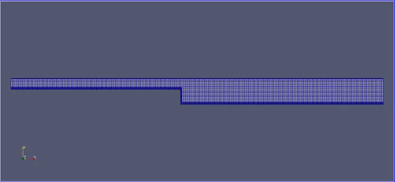
• Mesh Profile:

• Velocity contour

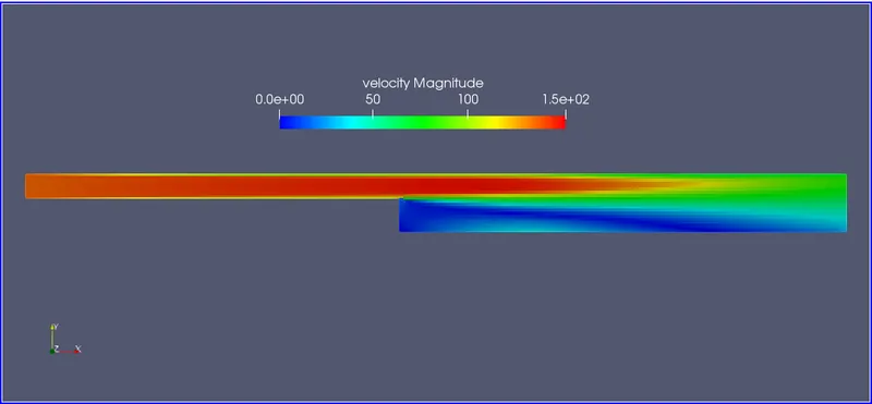
Approximately of 60 m/sec due to the increased in the geometry and at the step thevelocity is very low due to the divergent nozzle and the flow is turbulent so the pressuredroping takes places so that the velocity starts decreasing from this point only.

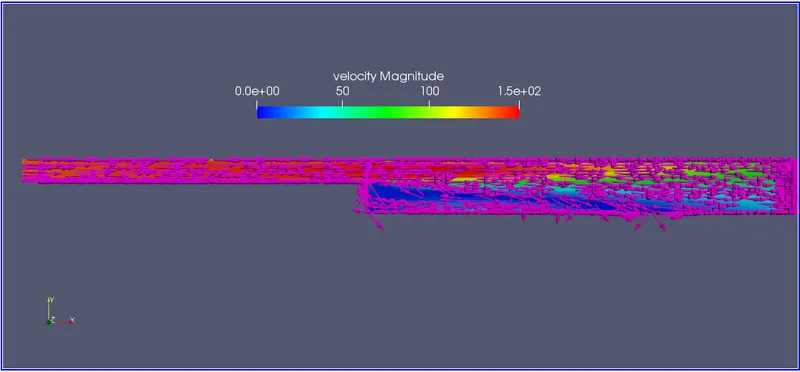
In the velocity counturs with the vectors the velocity after the step is recirculating becauseof the separation in the flow and form the boundary layer with the shear zone and atdistance forming a vortex which is the region for recirculating the flow.

• Velocity animation

• Velocity plot

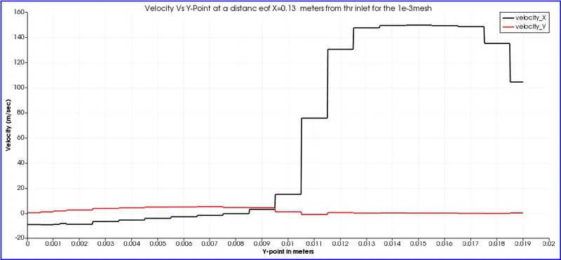
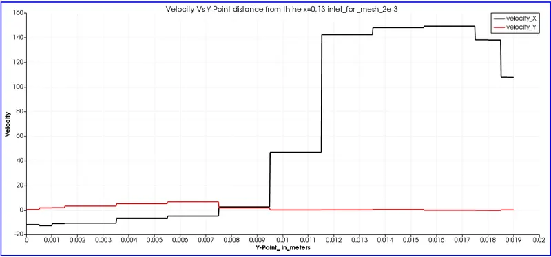
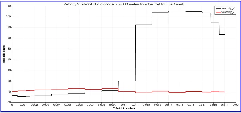
From this graph we observed that the velocity of the flow is low in the step region beacuseof the flow is turbulent and the velocity is changed enormously from the point 0.015 metersand reached the highest velocity of 150 m/sec in the middle where we can observe graphas it rises after that decrease in the velocity at the wall region.

• Pressure contour

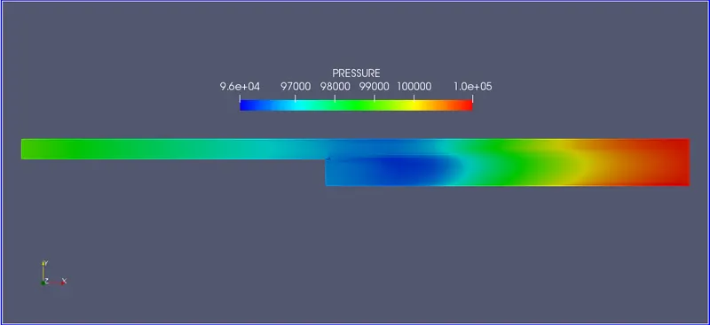
Initially the pressure is high at the inlet and it goes on increasing utill it reaches the stepregion and after that the pressure gradually changed it becomes lower in the step regiondue to the turbulence,the flow experiences an adverse pressure gradient, which causes theboundary layer to separate from the solid surfaces and after that there is a tremendousgrowth in the pressure untill it reaches the outlet and attains the maximum pressure.

• Pressure animation

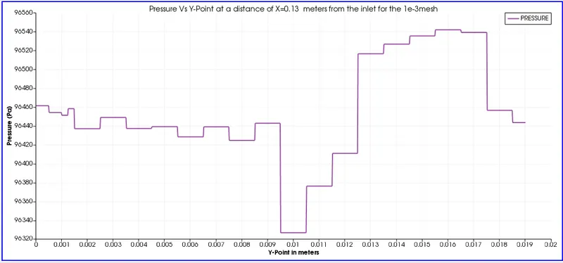
• Pressure plot

• Mass flow rate

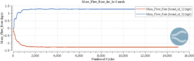
The mass flow rate is same for both inlets and outlets they are liked mirror image.Theconvergence is achieved after the 7000 cycles and value for the mass flow rate is 1.35kg/sec.

• Total Pressure at the inlet and outlet

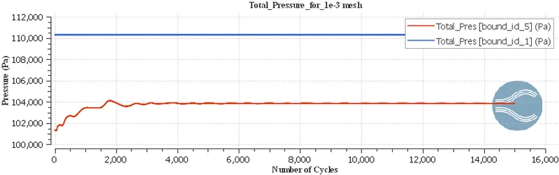
The pressure is constant at the inlet and the pressure at the outlet is gradually increasedfrom the starting cycles and achieved the convergence after the 8000 cycles and reaminsthe same value throughout the simulation.

• Average velocity at the inlet and outlet

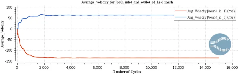
The Velocity at the inlet is -140 m/sec and the velocity at outlet is 60 m/sec.The velocity ishigh in the inlet and low at the outlet because of the increased cross sectional area for theoutlet when compared with the cross sectional area of the inlet.

• Total cell count

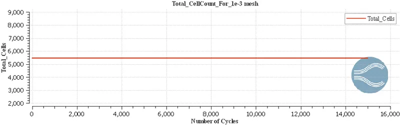
The total number of cells is around 5500 cells.The number of cells are increased beacuseof the more refinement of mesh and the outputs of all graphs and plots are smooth and fine.

Conclusion:

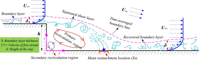
velocity profile for 1e-3 mesh

Backward flow

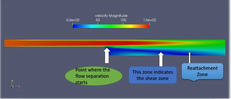
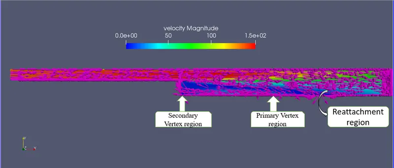
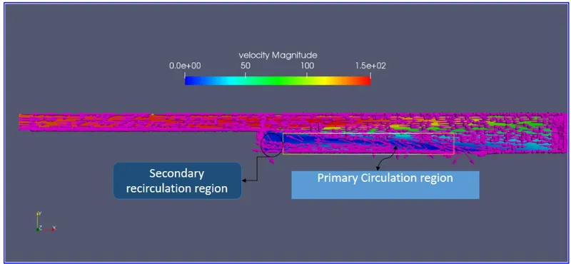
From the above images we can observe the general characteristics of the flow beginswhere the upstream boundary layer develops and the pressure gradient is developed intothin shear layer.

The turbulent structures in the shear layer catches the irrotational fluid from the nonturbulent flow and this causes from the low velocity recirculation in the region.

The primary vertex is accured at the center from the step and the secondary vertex isformed at the corner of the step and the pressure gradient forms the shear layer curves(inthe velocity image the sky blue color) goes down the wall and touches the wall.Some of thestreams flow right and forms the recirculation region and some them goes right andreaches the outlet.

The reattachemnt length is the distance between the step and the reattachmentpoint.After the both recirculation of flow occurs it flows towards the outflow direction inorder to discharge from the channel