Week 3: Flow over a backward facing step

Aim- Flow over a backward facing step

Introduction – In this task we will learn about importance backward facing step phenomena in field of CFD. Sudden change in in pipes will impact the fluid flow which can be disconitnuity in fluid stream , bubble formation and chnages in some paramteres contours.

In this task we will run the simulation for three different size grid and and will compare the pr plots , velocityplots , pr and velocity contour for better study .

Steps –

1. Geometry
2. Define the boundary
3. Case setup
4. Simulation
5. Post processing
6. Outputs
7. Conclusion

Geometry –

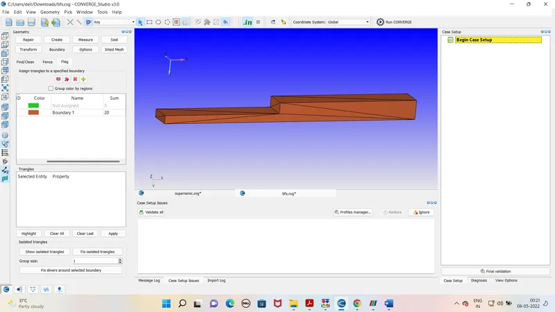
1. Import the geometry in the converge software .

2. Define the boundaries for inlet , outlet, top , bottom , front and back.

3. diagonsis the geomtery for any errors.

Case setup –

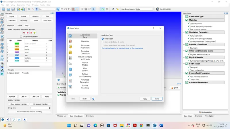
Application type –

Pre defined mixture - Air

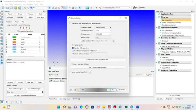
Gas simulation –

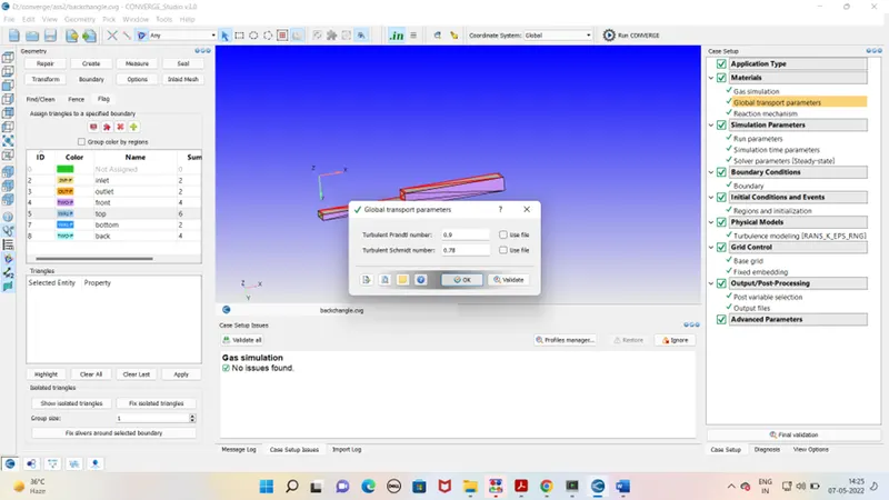
Global transport parameter –

Reaction meachinsm

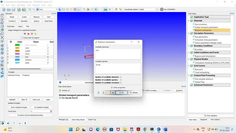
Simulation Parameter –

Run parameter –

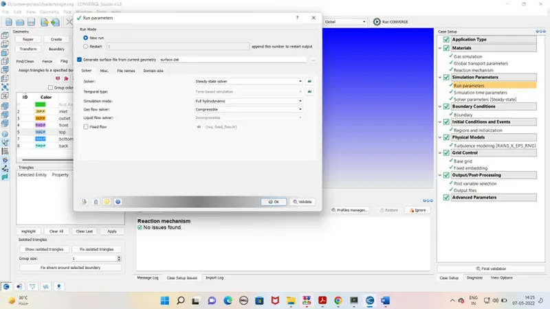
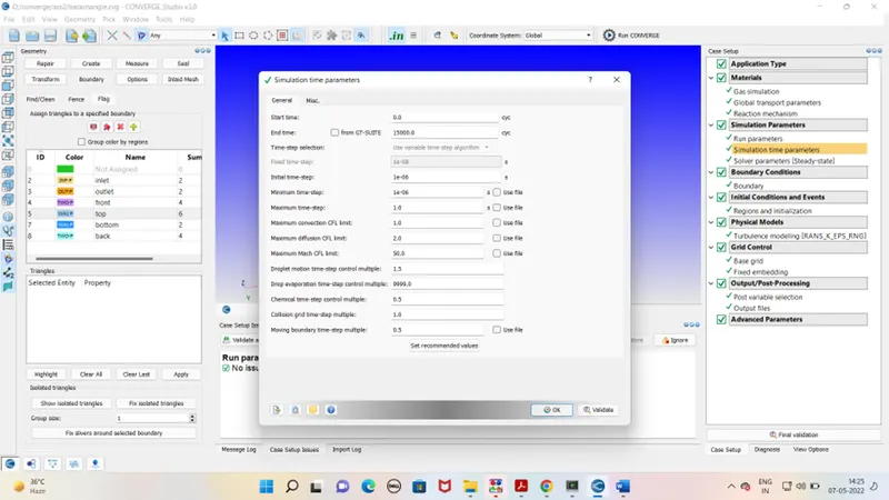
Simulation time parameters-

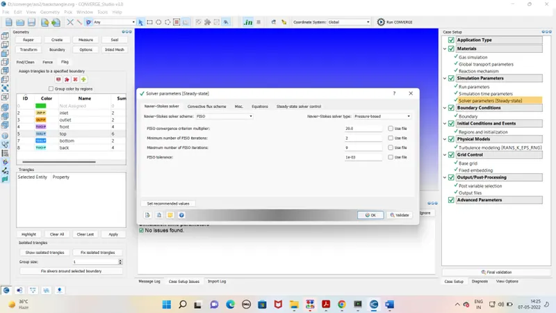
Solver parameters-

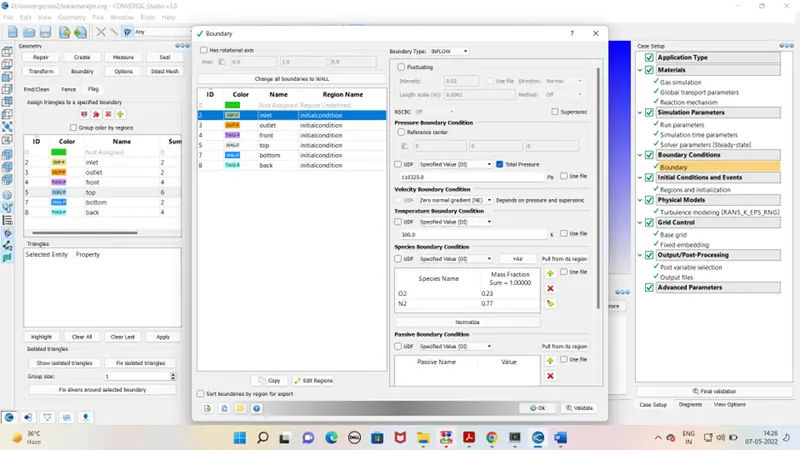
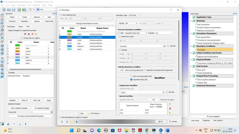
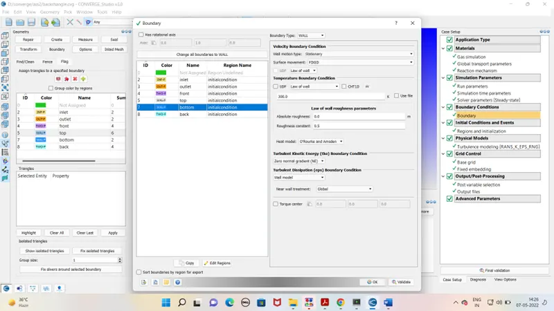
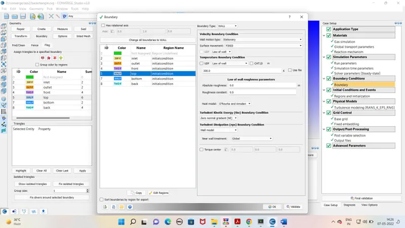
Boundary condition –

Inlet

Outlet

Define Front and back side as 2D boundary type –

Top and bottom wall –

Intial condition and events –

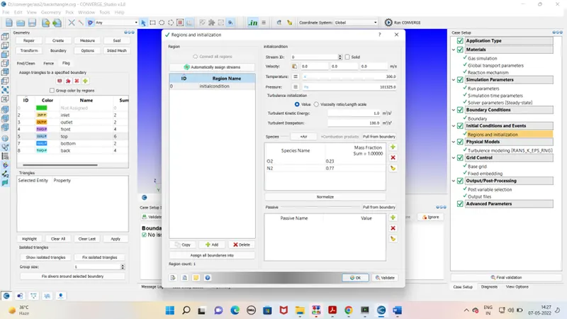
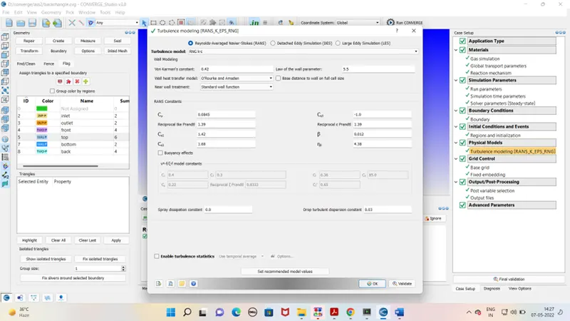
Physical models –

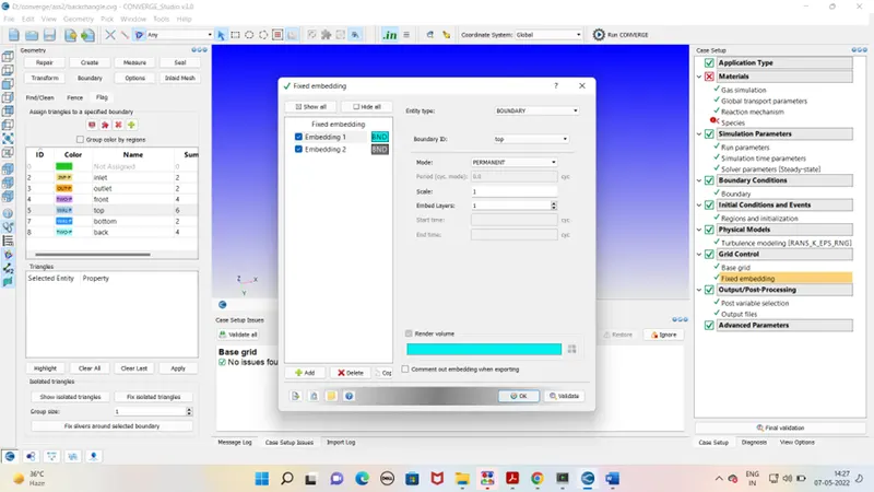
Grid control –

Case 1 - Base grid – dx - 0.002 dy –0.002 dz – 0.002

Case 2 - Base grid – dx - 0.0015 dy –0.0015 dz – 0.0015

Case 3 - Base grid – dx - 0.001 dy –0.001 dz – 0.001

Fixed embedding -

Output processing Advanced parameter –

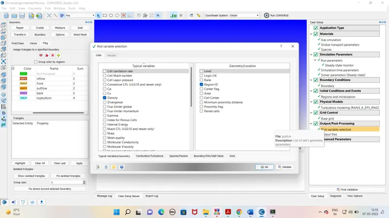
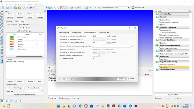
After case set up exports the file to defined folder. Run the simulation in the Cygwin. Generate the output files. As output file is generated run the post processing in Cygwin again. Open the output file in paraview for the mesh view and contours. For excessing pressure , velocity and mass flow rate use line plotting tab.

Outputs –

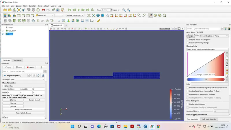
For grid size – 0.002

Mesh -

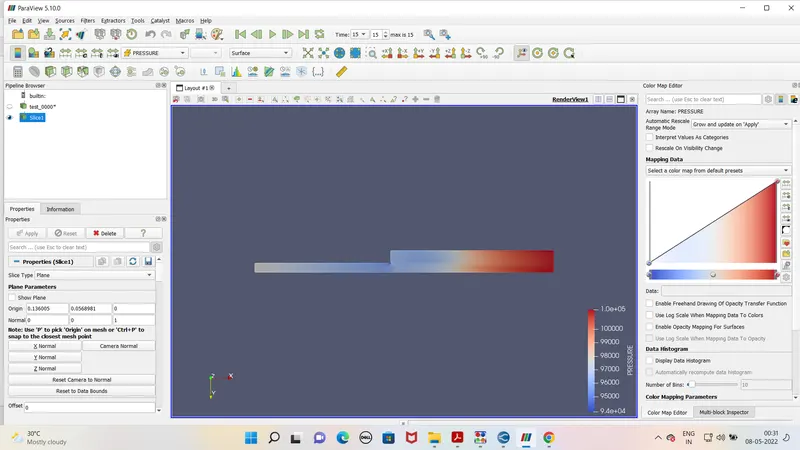
Pressure contour -

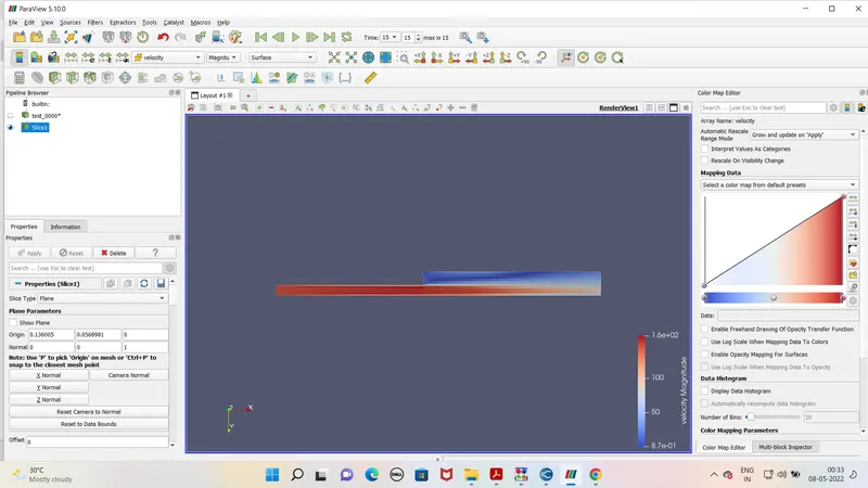
Velocity contour-

For grid size - .0015

Mesh

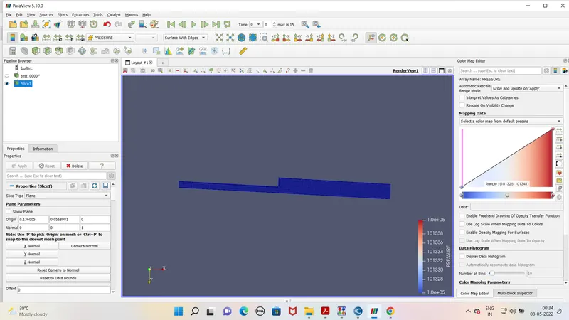
Pressure contour -

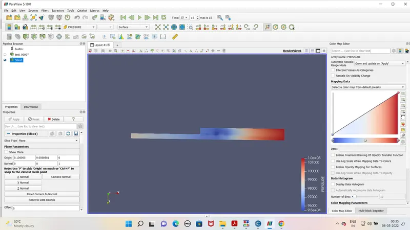
Velocity contour -

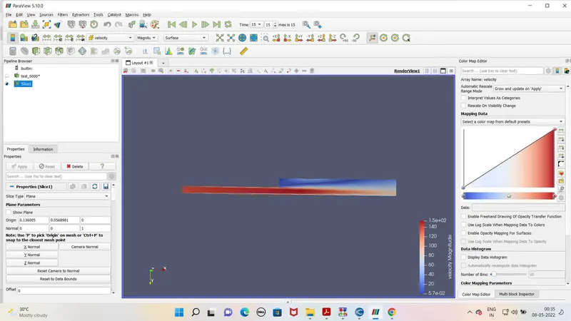
For grid size – 0.001

Mesh

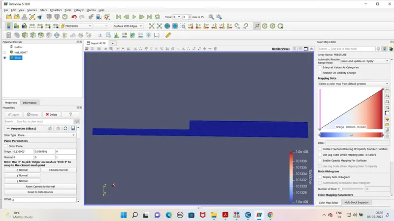
Pressure contour -

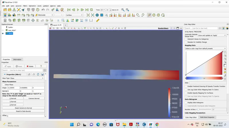
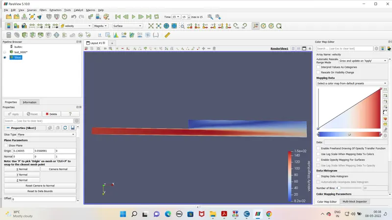
Velocity contour -

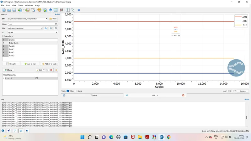
Total cells -

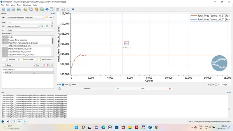
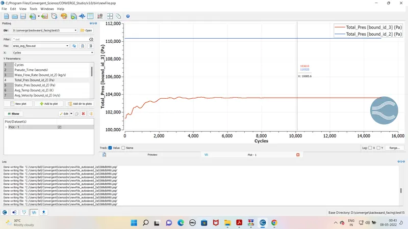
Pressure plot for 0.002

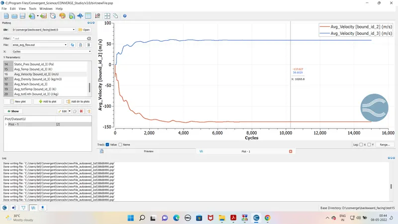
velocity plot for 0.002

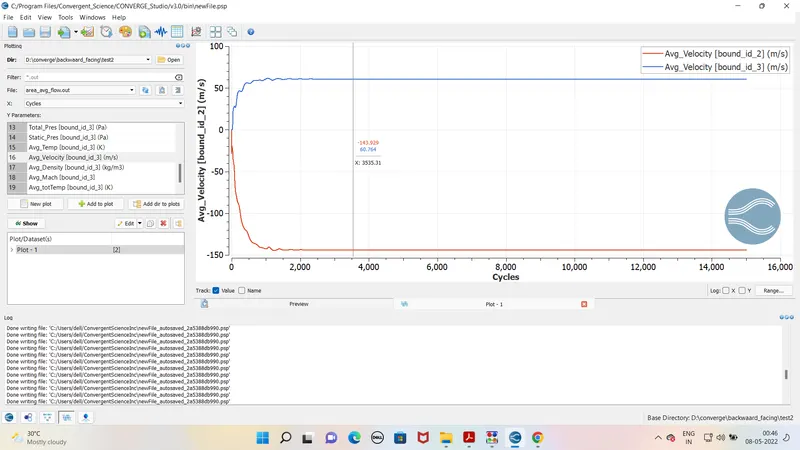
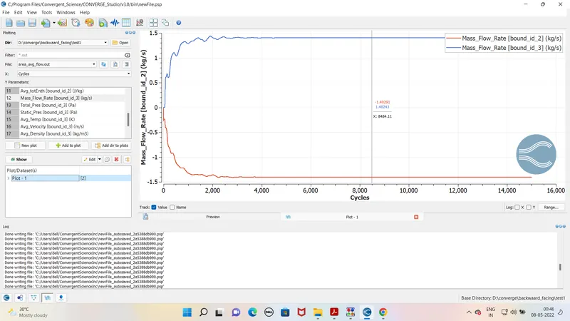
mass flow rate plot for 0.002

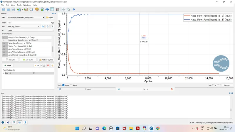
Pressure plot for 0.001

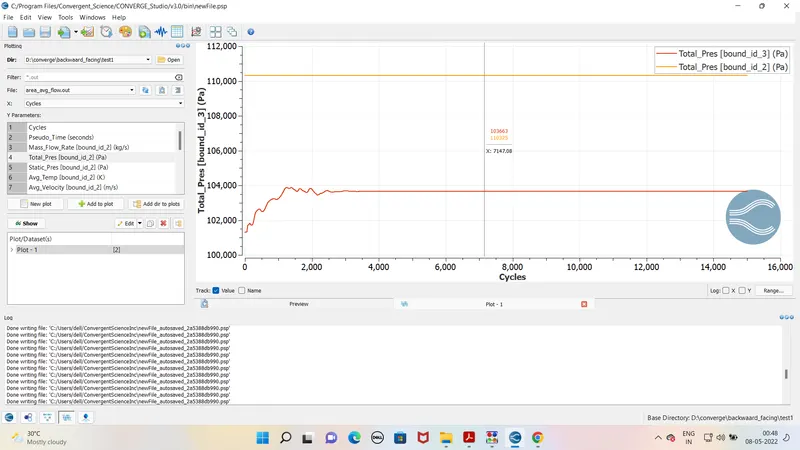
velocity plot for 0.001

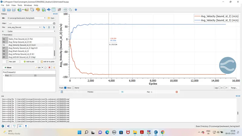
mass flow rate plot for 0.001

Pressure plot for 0.0015

velocity plot for 0.0015

mass flow rate plot for 0.0015

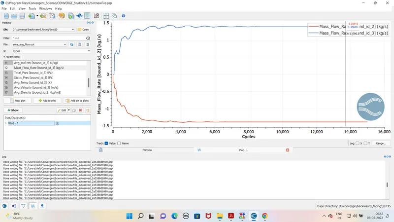
Conclusion –

1. From the above results it is noticed that as we reduce the mesh size the conotur results appear more clear . Same it will take take more time for simulation.

2. From above contours it is seen that velocity flow in entry was equally disctributed along the boundary but as there is sudden change in shape in geometry it is noticed the zero velocty region created, and at end outlet end as area inc the pr increased and velocity reduced to minimum.

Remarks -

Due to slow net i am unable to upload animations.