Week 3: Flow over a backward facing step

OBJECTIVE: To Simulatea flow over backward facing step

THEORY: Backward facing step flow is widley used in industrial testing to verify the CFD simulations model created before actually testing them on the main parts/models/bodies so as in order to verify the accuracy of the CFD simulation model, as we have a lot of experimental data available in regards with backward facing step flow we can easily verify simulation results with experimentals results and can gain confidence in the CFD simulation model created. We see a flow sepration in the model due sudden changes in the cross sectional area available for fluid flow and also due to the difference of pressure at inlet and outlet. This flow sepration generates point of recirculation and point of reattachment.

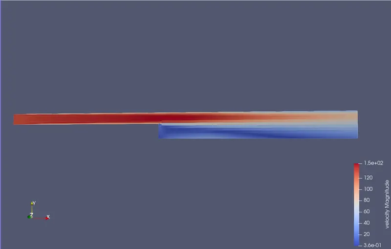
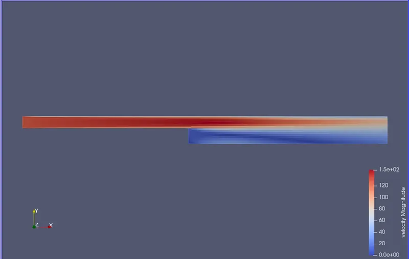
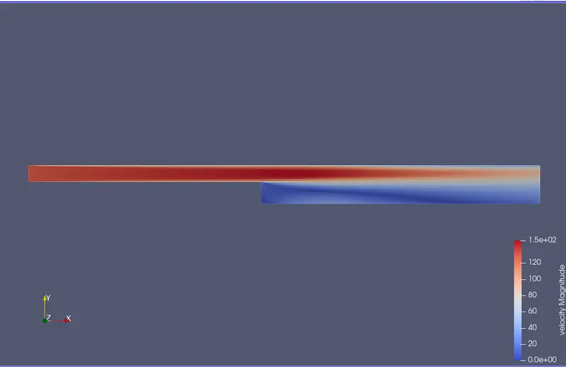
In our model the fluid enters from left hand side of the model and as soon it reaches the step region we see a flow sepration region where the fluid starts to recirculate in the region and a swirl like motion can be seen in that region of the fluid flow and completing the recirculation the fluid reattaches with the main stream flow resulting in increased velocity of the fluid flow.

SIMULATION SETUP / PROCEDURE: We start our simulation by creating the model of backward facing step using simpple create tools of CONVERGE STUDIO. After creating the model each side/face of the model is assigned boundaries accordingly and appropriate names are given to them. After this we go ahead to setup the case setup tree which is obtained by clicking begin case setup, our application type is selected as time-based simulation.

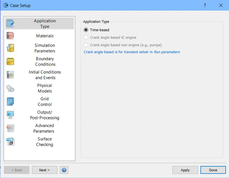
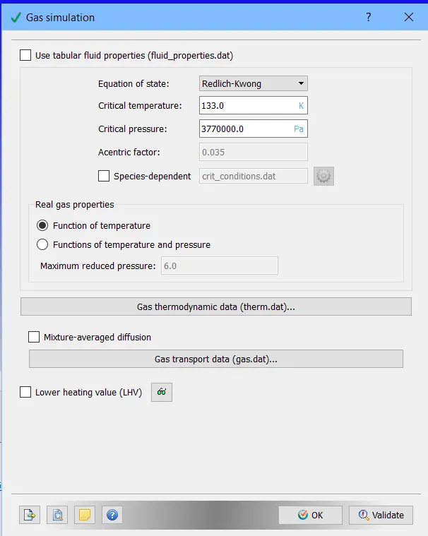
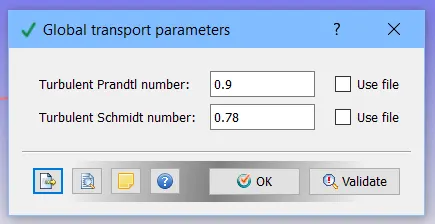
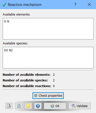
For materials pre-defined material was selected to be air and reacton mechanism was enabled also the gas simulation setup, global transport parameters and reaction mechanism were validated with their default values.

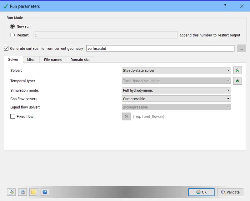
After this we setup our Run parameters where solver type was selected to be steady-state and simulation was set to full hydrodynamic and gas flow solver was set to compressible.

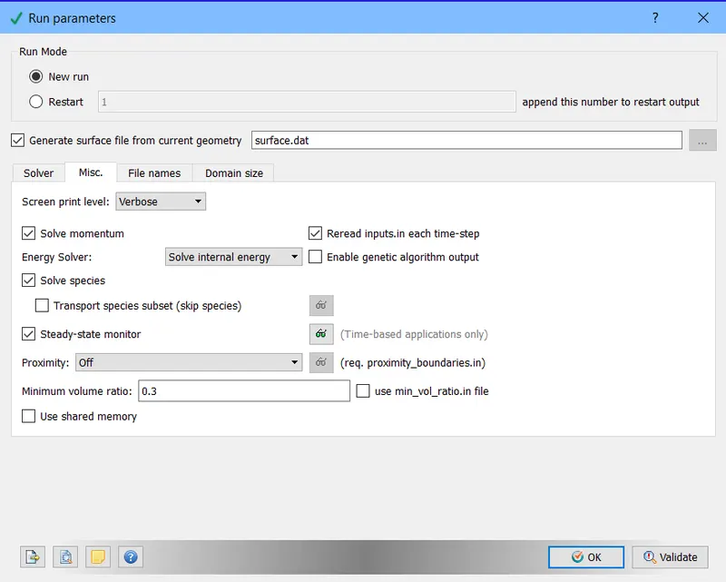
Also use shared memory was disabled and simullaion monitor was enabled.

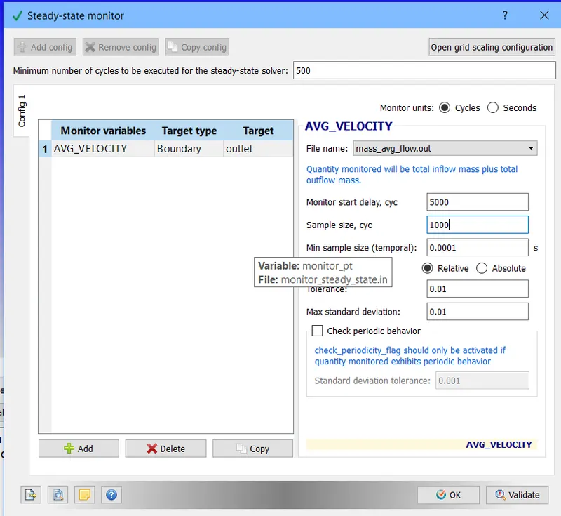
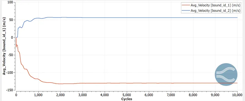
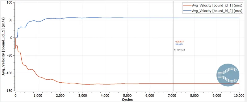
After this we setup steady-state monitor by giving in the required values the monitor variable was set to avg velocity.

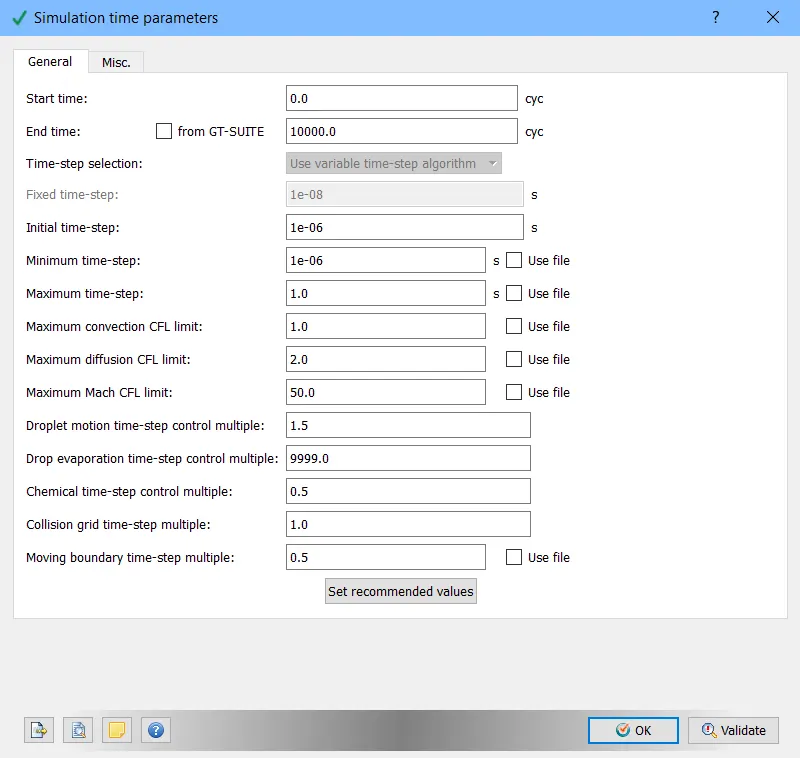
After thiswe setup simulation parameters where we set the initial time step to be 1e-6 also this was our minimum time step and max was set to 1. rest values were set to default.

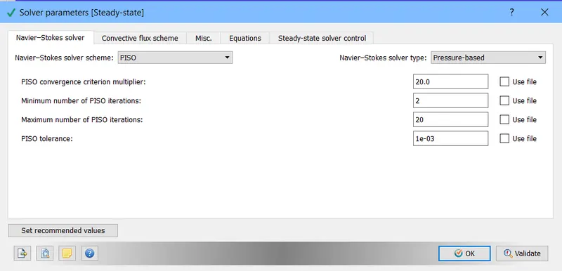
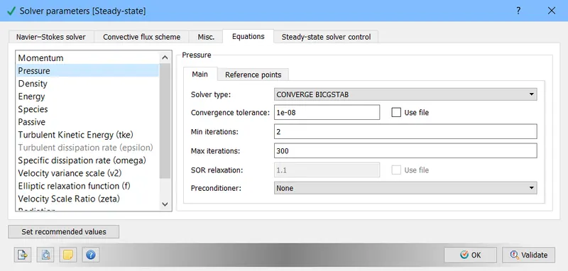
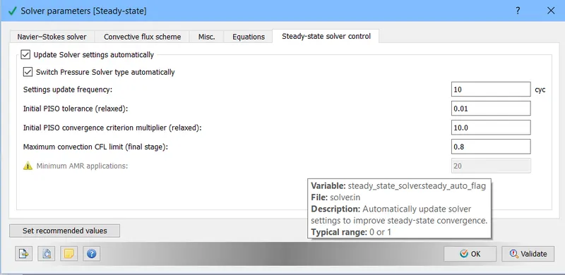
After we setup solver parameters, where PISO scheme was applied using pressure-based method. And pre-conditioner for pressure was set to none. Maximum CFL limit was set to 0.8

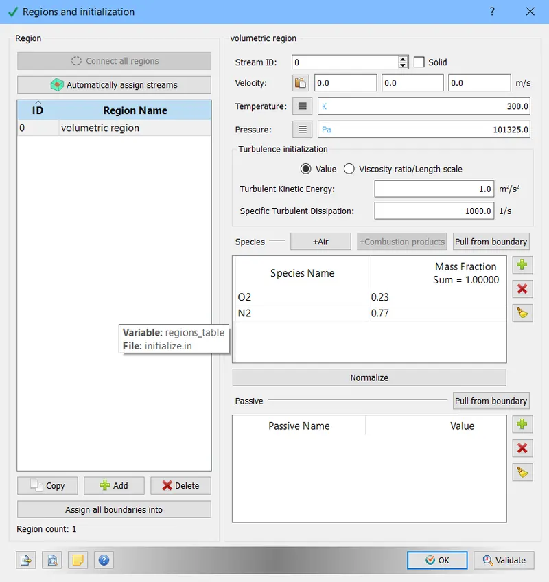
After this we defined a region named volumetric region.

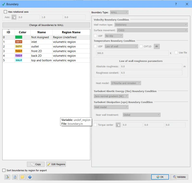
After seeting up the region we go and setup our boundaries and assign them regions.

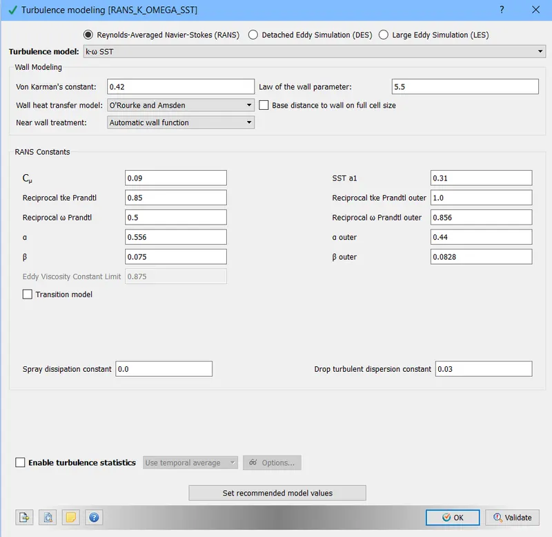
After this we setup our tubulence model where we choose k-omega SST.

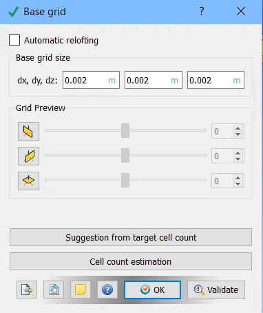
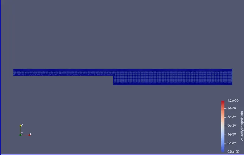
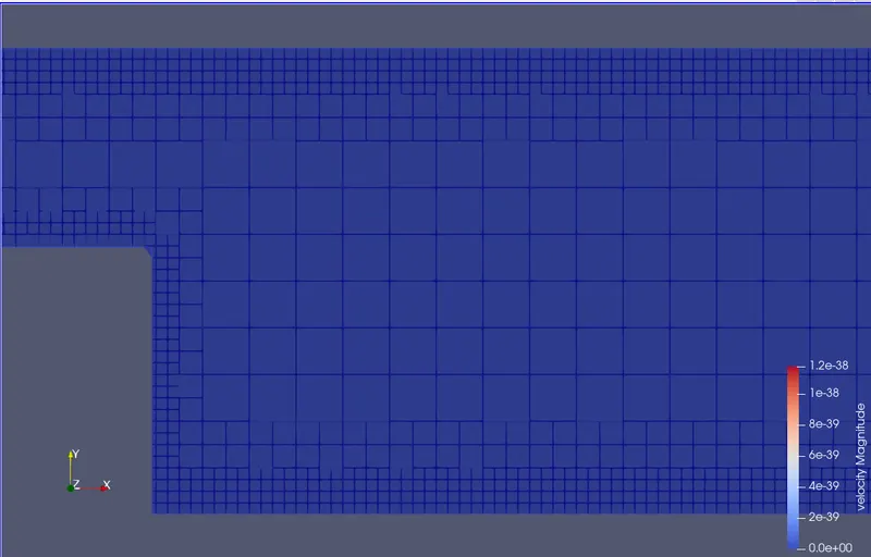
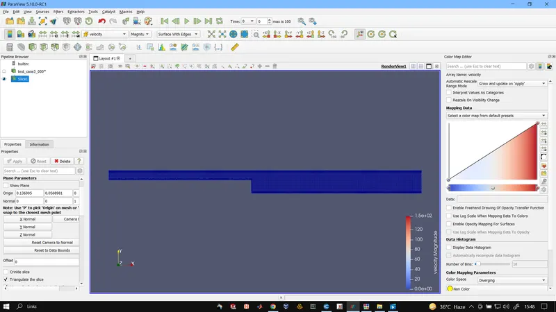
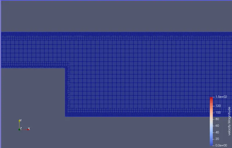
After this we setup our base grid sizes and enable fixed embedding and set it to scale of 2 for 2 layers and embeeding type was surface and duration was permanent.

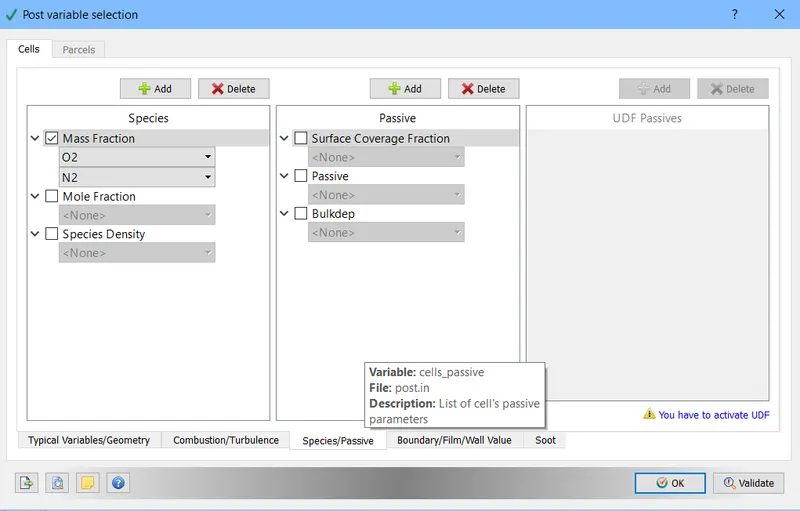
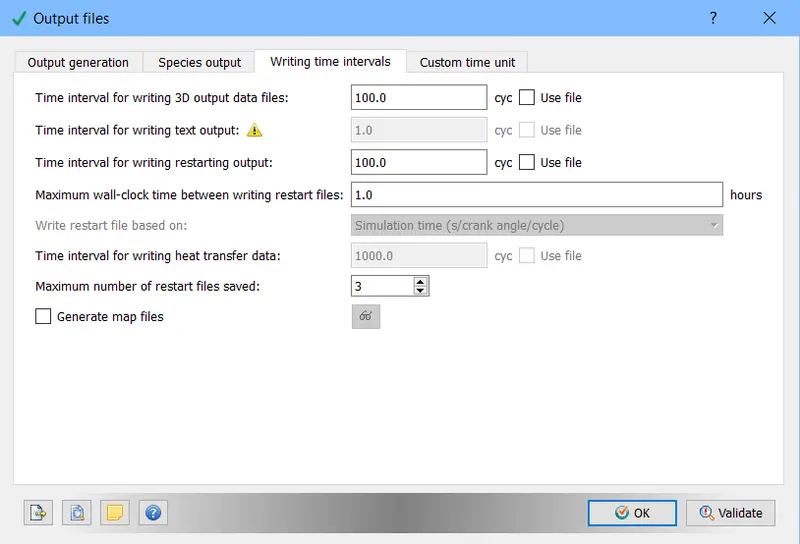
After this we setup our post variables and output files where we declare interval for writing output and restart files as well as number of restart files to generate.

RESULTS:

TEST CASE1 MESH SIZE 2e-3

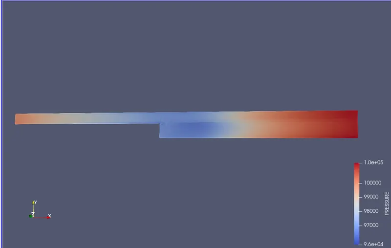
TEST CASE2 MESH SIZE 1.5e-3

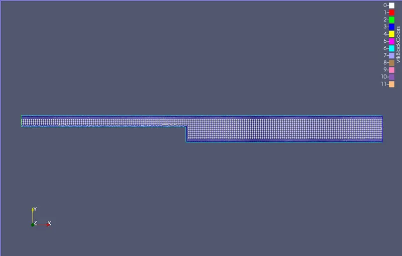
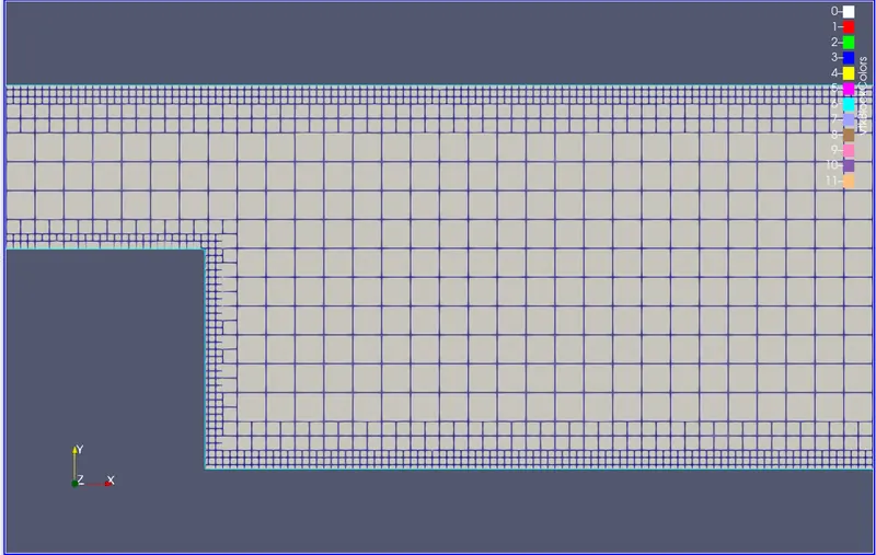
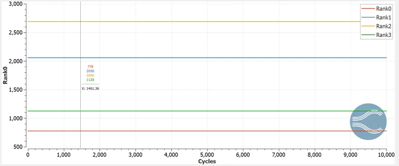
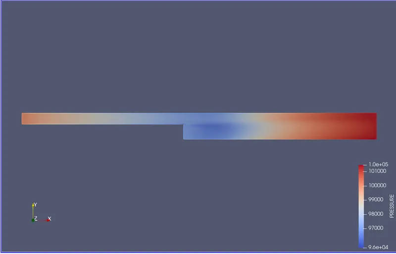
TEST CASE3 MESH SIZE 1e-3

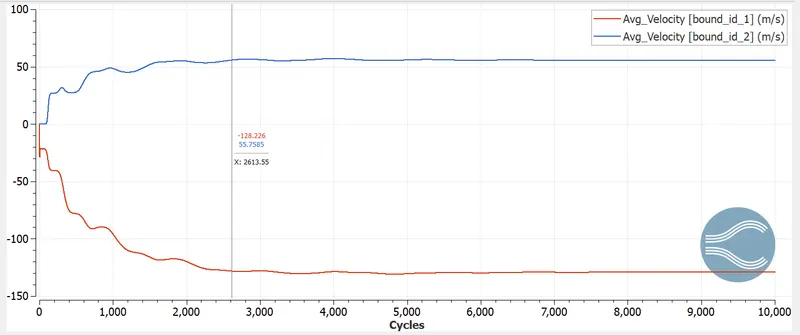
CONCLUSIONS:

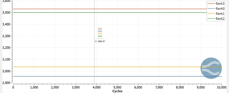
As the mesh gets finer we get more accurate results and better flow visualisation, fixed embedding helps us refine the mesh in the regions required without altering the base mesh resulting in better results on less cell counts.

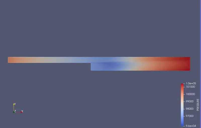
The flow separation occurs where the cross-section area for fluid flow increases and results in formation of eddie flow and due to this we have a turbulent flow and hence we used k-omega SST turbulent flow model.

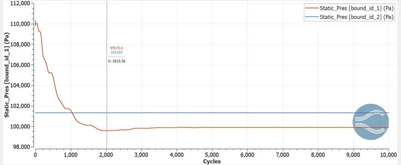
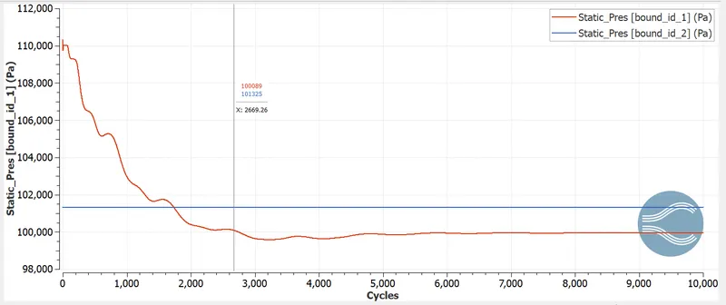
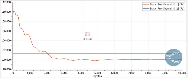
We observe pressure at inlet to drop while at outlet remains constant the drop in pressure is due to change in available area for flow.

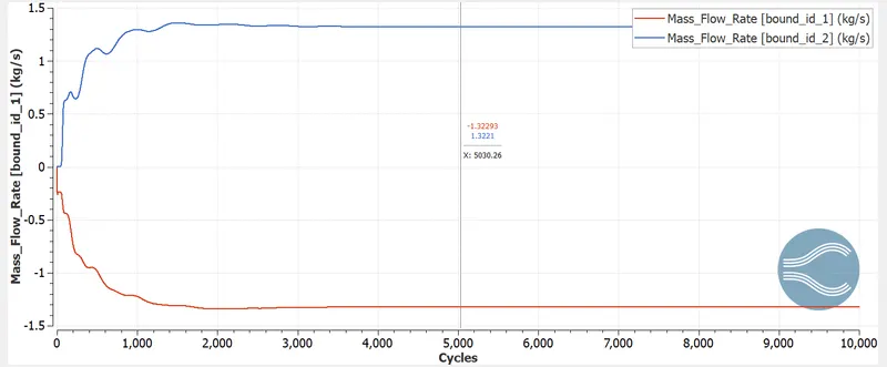
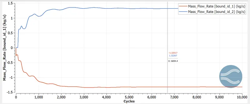
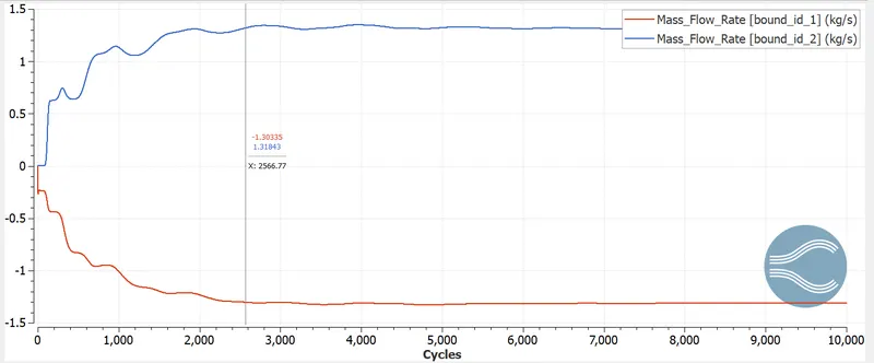
Mass flow rate plots show that the mass conservation is implied in the system.

We have maximum velocity in the upper region of the step as the reirculation flow when attaches with main flow it increases its speed even furhter.