Week 3: Flow over a backward facing step

Aim:

• To simulate the flow over a backward step for three different mesh grid sizes by using the Converge CFD software, Cygwin and Paraview.
• To show various velocity and pressure contours for the different mesh.
• To show the various plot of velocity, pressure, mass flow rate, and total vell count for different mesh grids.
• To steady the turbulent flow characteristics in the flow over a backward step.

Introduction:

What is the Backward Facing Step?

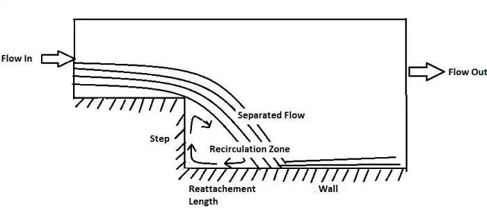
Figure: Flow features of Backward facing Step flow

Fully developed flow enters the domain from left. When the flow reaches the step, because of expansion of flow channel, pressure gradient exists, it detaches and a recirculation zone is formed. A turbulent boundary layer encounters a sudden back step, causing flow separation. Later the flow eventually reattaches to the bottom wall.

Backward-Facing Step (BFS) flow is one representative model for separation flows, which can be widely seen in aerodynamic flows (airfoil, spoiler, high attack angle process), engine flows, condensers, vehicles (cars, boat), heat transfer systems, and even the flow around buildings, etc. The flow separation after a simple stage will introduce separation bubble formation, evolution and re-attachment process, which is dependent on the Backward Facing Step geometric design, the inlet and outlet conditions, turbulent intensity, as well as heat transfer conditions. It is shown that the step size (duct expansion ratio) will define the basic re-circulation and re-attachment process.

It is a basic model involving the most important feature of a separated flow –a free shear flow separation, vortex generation and reattachment.

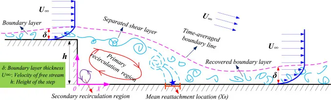
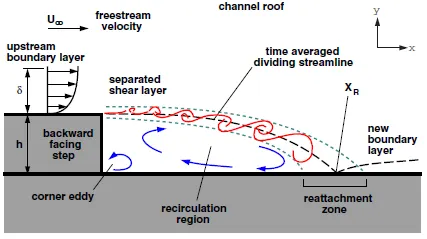
A backward step flow includes an inflow of uniform velocity,laminar or turbulent from a channel to a step on the either sides with a step height of h .The flow fluid is divided into four regions namely separated Shear layer ,the recirculation region under the shear layer,the reattachment region, and the recovered boundary layer.

Flow with separation and reattachment has long been a subject of fundamental fluid dynamics research. The presence of a separated flow, together with a reattaching flow, gives rise to increased unsteadiness, pressure fluctuations, structure vibrations and noise, as it also exhibits an unsteady structure with a large scale vortex in the separated shear layer and low-frequency motion around the reattachment region with fluctuation of an instantaneous reattachment point.

Turbulent flow over a backward-facing step is one of the classical tests to validate turbulence models in CFD. In the present work, steady-state turbulent flow over a backward-facing step was simulated using Converge with the Renormalization-group (RNG) k-ε model to account for turbulent viscosity

Turbulent flows occur in a variety of industrial problems. A flow is termed as turbulent when the inertial forces of the fluid are greater than the viscous forces resulting in chaotic fluctuations in the flow.

Importance of Backward Facing Step Problem

Separation and reattachment of turbulent flows occur in many practical engineering applications. It is seen both in internal flow systems such as diffusers, combustors and channels with sudden expansions, and in external flows like flow around airfoil and building. In these situations, the flow experiences an adverse pressure gradient, which causes the boundary layer to separate from the solid surface. The flow subsequently reattaches downstream forming a recirculation bubble. The presence of a separated flow, together with a reattaching flow, gives rise to increased unsteadiness, pressure fluctuations which may lead to structure vibrations and noise.

Procedure for the Generation of Geometry:

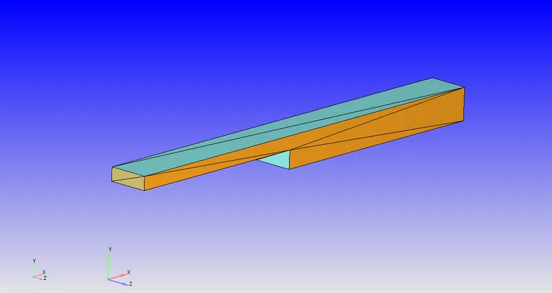
The length of the backward_facing channel is 0.272m, and the dimensions of the inlet and outlet are 0.01m and 0.02m respectively. Since, we are performing a 2D simulation on the given backward-facing step, the length of the channel in the z-direction is not important.

Moreover, we have given names to different faces of the geometry(inlet, outlet, front, back, top and bottom boundaries.

Case Setup

1. Mesh sizes:

Mesh element sizes in x-y and z-directions:

Case 1 - 2e-3

Case 2 - 1.5e-3

Case 3 - 1e-3

2. Type of simulation: Steady state simulation with zero reactions and only air(77% N2, 23% O2) as the medium of flow.

3. Steady-state monitor properties:

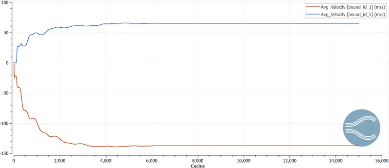
a) Average velocity at the outlet

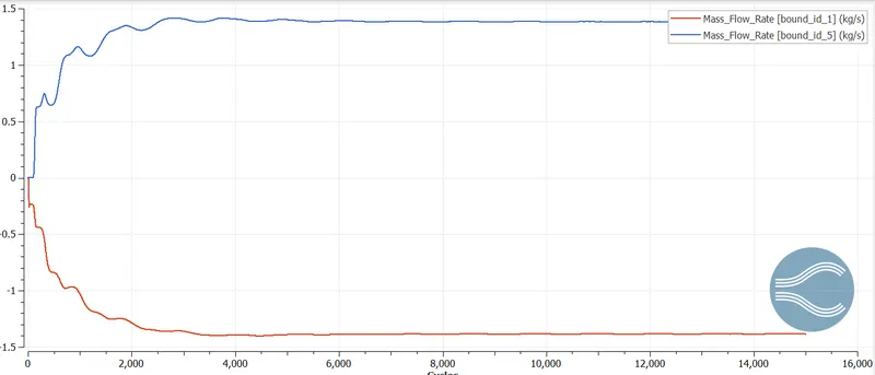
b) Average mass flow rate at the outlet

4. Boundaries:

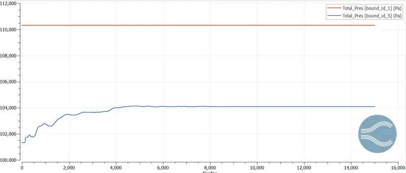
Inlet: Inflow boundary condition with pressure inlet (110325Pa) and temperature (300K).

Outlet: Outflow boundary condition with pressure outlet (101325Pa).

Top and Bottom: Stationary, no-slip wall.

Front and Back: 2D faces.

Pressure difference between the inlet and outlet = 9000Pa

5. Solver properties:

Details: 2 minimum iterations and 20 max iterations per cycle. Tolerance = 0.001

Minimum Cycles = 0

Maximum Cycles = 15000

Minimum time step = 1e-9 sec

Maximum time step = 2.0 sec

Maximum convection CFL limit(final stage)= 1.0

6.Turbulence model:

RNG K-epsilon turbulence model

7. Results:

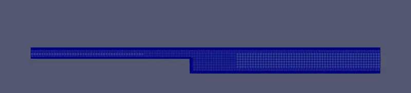
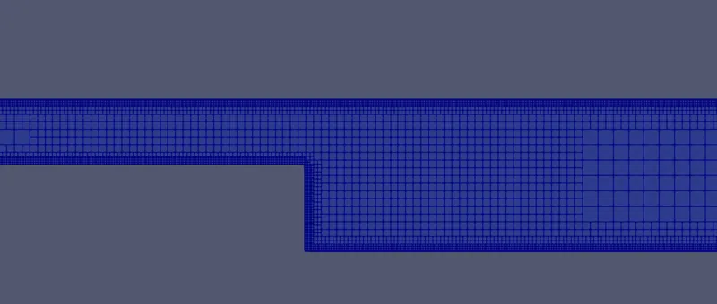
Case 1: Mesh grid size = 2e-3m

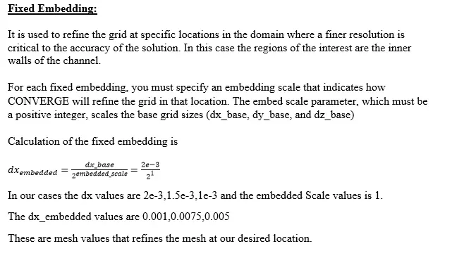
Fixed Embedding:

At top and bottom boundaries - Scale factor - 3, Embed layers - 3

At the step - Box boundary

Mesh:

Velocity Contours:

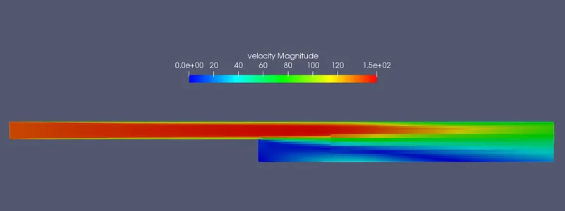
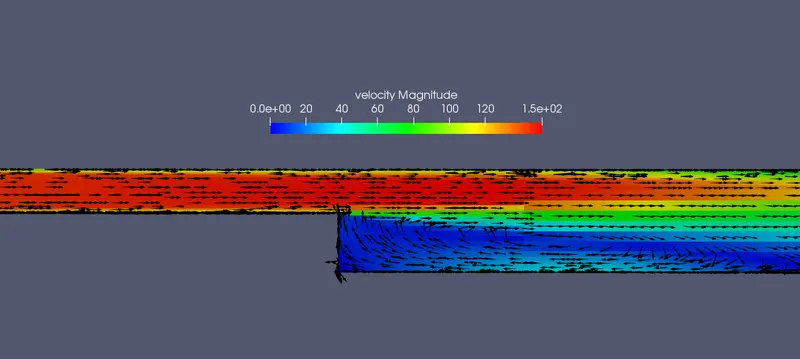
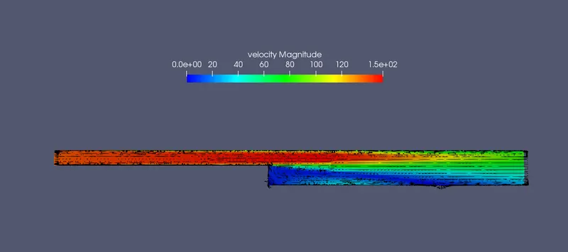
Link for animation video - https://drive.google.com/file/d/1RCHggZTDOHtoyKJlBJYgeougnNvLLQgL/view?usp=sharing

Pressure Contours:

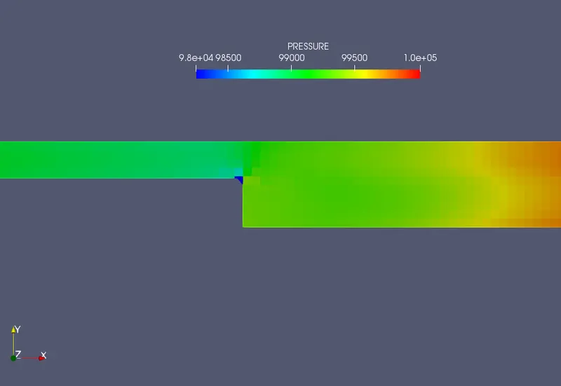
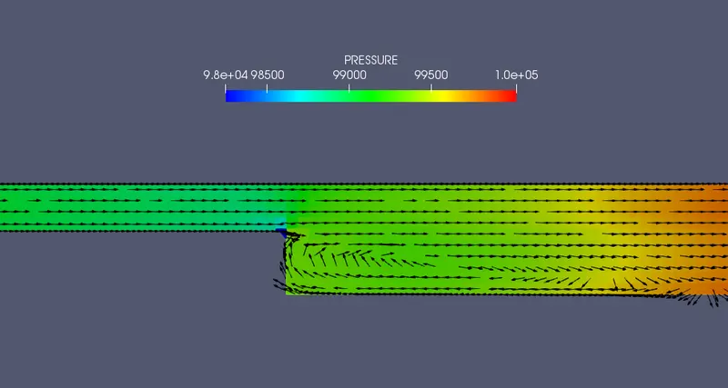
Link for animation video - https://drive.google.com/file/d/1CknMzO81iDDfTNzOIYP0lyeP1B54y6TI/view?usp=sharing

Line Plots:

Average Velocity:

Total Pressure:

Mass Flow Rate:

Cell Count:

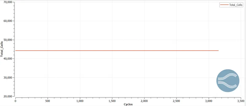
The total number of cells is 989.

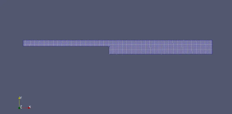
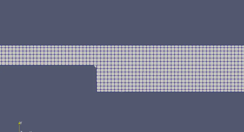
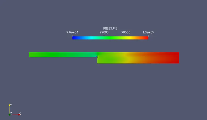
Case 2: Mesh grid size = 1.5e-03 m

Mesh:

Velocity Contours:

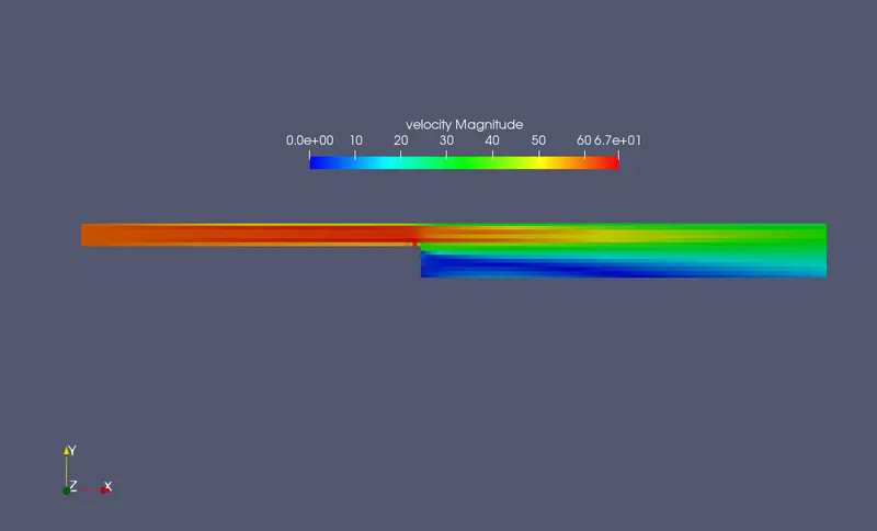
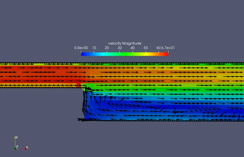
Link for animation video - https://drive.google.com/file/d/1awDuqOjmHjo3tRpI7Rkrtc2tVfrfbEoC/view?usp=sharing

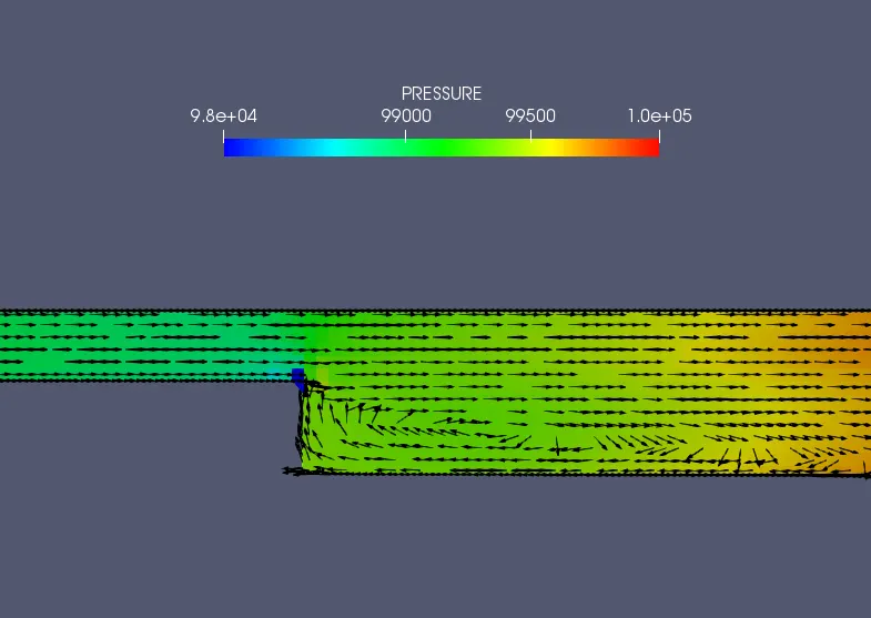
Pressure Contours:

Link for animation video - https://drive.google.com/file/d/1OO2S9yMU2YNZOeO8hJekDES-WMHlbXPr/view?usp=sharing

Line Plots:

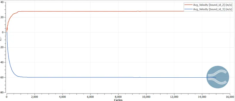
Average Velocity:

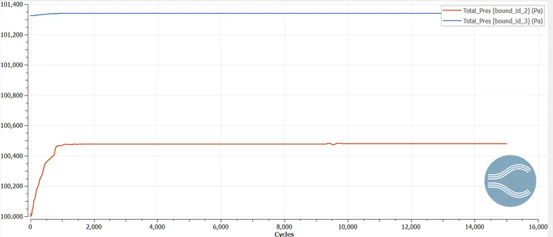
Total Pressure:

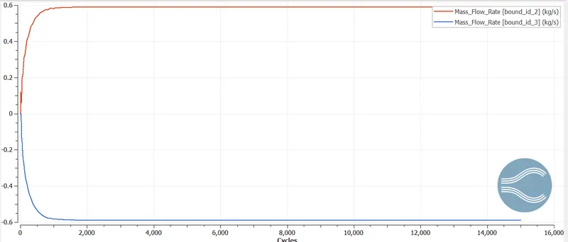
Mass Flow Rate:

Cell Count:

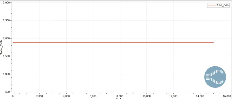
The total number of cells is 1884.

Case 3: Mesh grid size = 1e-03 m

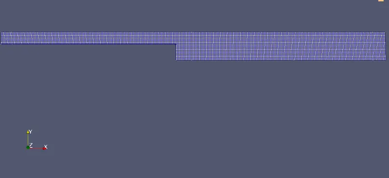
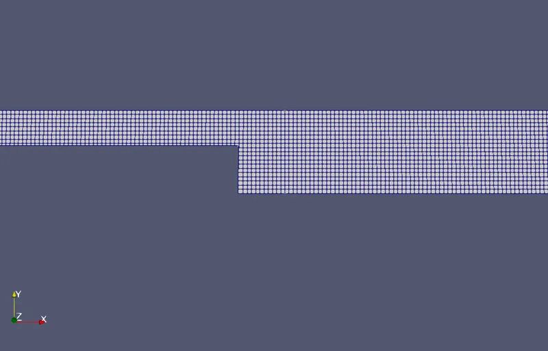
Mesh:

Velocity Contours:

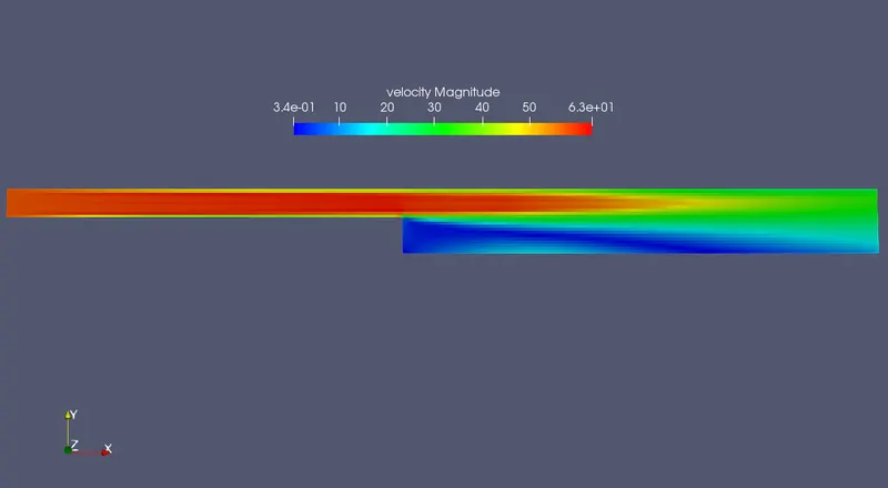
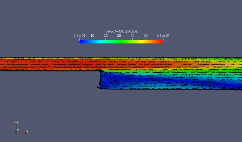
Link for animation video - https://drive.google.com/file/d/1P3O81u0FUbWNRSzwHl9RgXq1UJsySodf/view?usp=sharing

Pressure Contours:

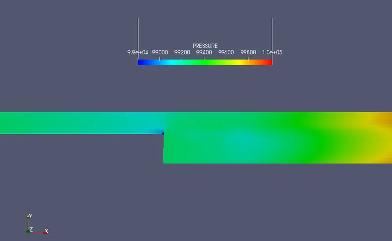
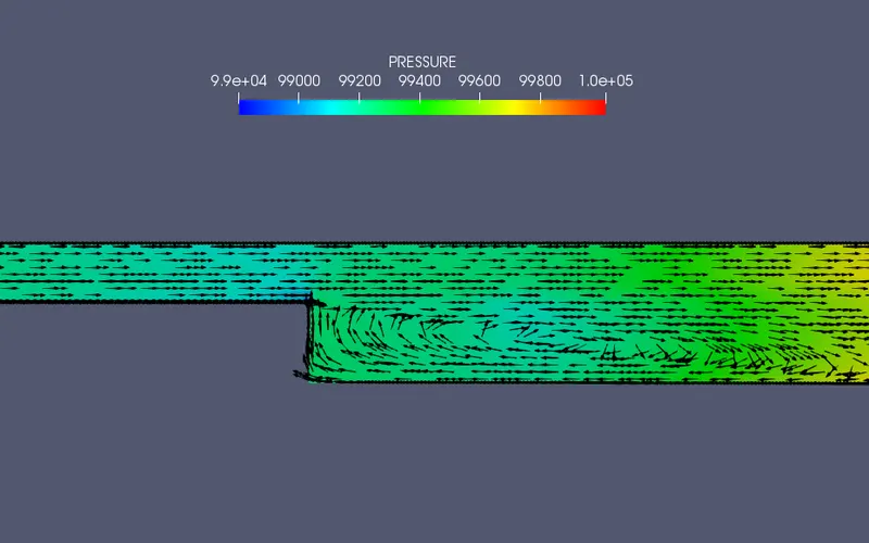
Link for animation video - https://drive.google.com/file/d/12wUj93uqTpjO9Ag6hFNKpifl0sw5jyh8/view?usp=sharing

Line Plots:

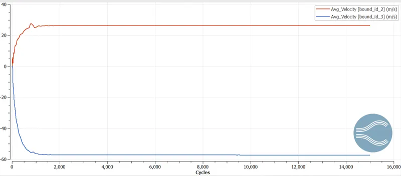
Average Velocity:

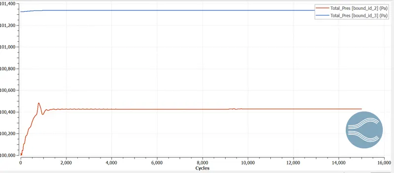
Total Pressure:

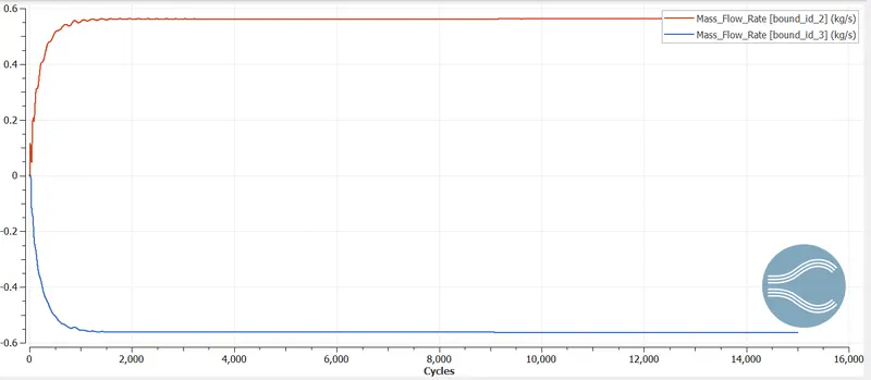
Mass Flow Rate:

Cell Count:

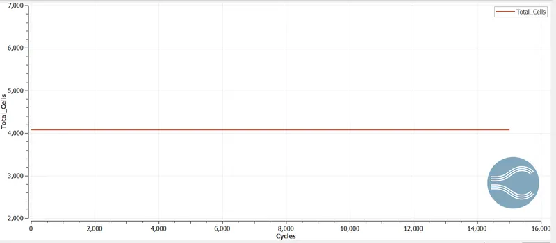
The total number of cells is 4076.

Conclusion:

The flow simulation of air was performed on the backward-facing step for 3 different mesh sizes and the following conclusions can be drawn:

1. The air flows from the inlet to the outlet. The velocity of air is higher at the inlet than at the outlet. This is because of the backward-facing step, which changes the geometry of the fluid domain.
2. Due to the backward-facing step, there is a pressure drop near the step, this causes some fluid particles to flow in the reverse direction, which creates vortices. This can be clearly seen in the vector plot.
3. With the increase in the number of grid elements, the solution obtained becomes more and more accurate. The flow properties are captured more accurately if the mesh is more refined. This is the reason for the introduction of embedded layers which improves the accuracy of the solution near the walls. In general, the smaller the element size, the more accurate is the solution obtained.
4. With the increase in the number of cells, the solution becomes more accurate but the computation time increases considerably. Hence, the problem must be studied thoroughly before performing the simulation and it must be decided how much are we willing to compromise the accuracy of the solution to save resources.