Project 2 - Rankine cycle Simulator
Aim:
- Create a Rankine Cycle Simulator using OCTAVE/MATLAB.
- Your code should calculate the state points of the Rankine Cycle based on user inputs.
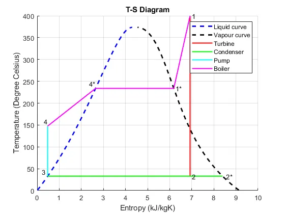
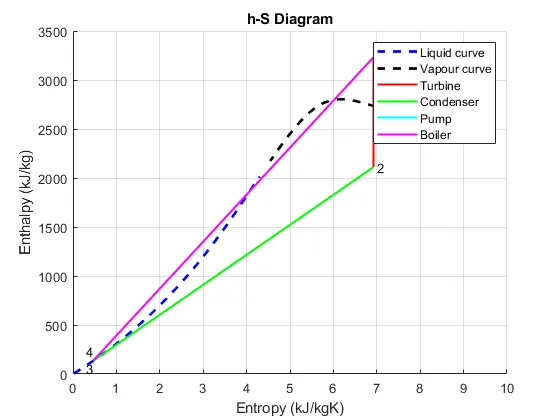
- Then, plot the corresponding T-s and h-s plots for the given set of inputs.
Input values:
- Turbine Inlet temperature = 400° C
- Turbine Inlet Pressure = 30 bars
- Turbine Outlet Pressure = 0.05 bars = Condenser Inlet Pressure
Required output values:
- Net work output
- Back work ratio
Introduction:
The Rankine cycle or Rankine Vapor Cycle is the process widely used by power plants such as coal-fired power plants or nuclear reactors. In this mechanism, a fuel is used to produce heat within a boiler, converting water into steam which then expands through a turbine producing useful work. This process was developed in 1859 by Scottish engineer William J.M. Rankine. This is a thermodynamic cycle which converts heat into mechanical energy—which usually gets transformed into electricity by electrical generation.
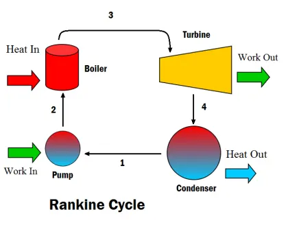
Figure 1. A simple schematic with components for the Rankine Cycle.
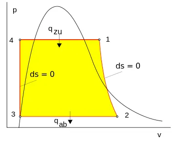
Figure 2. The pressure volume diagram of the Rankine cycle. This illustrates the changes in pressure and volume the working fluid (water) undergoes to produce work.
The steps in the Rankine Cycle as shown in Figure 1 and the corresponding steps in the pressure volume diagram (figure 2) are outlined below:
Pump: Compression of the fluid to high pressure using a pump (this takes work) (Figure 2: Steps 3 to 4)
Boiler: The compressed fluid is heated to the final temperature (which is at boiling point), therefore, a phase change occurs—from liquid to vapor. (Figure 2: Steps 4 to 1)
Turbine: Expansion of the vapor in the turbine. (Figure 2: Steps 1 to 2)
Condenser: Condensation of the vapor in the condenser (where the waste heat goes to the final heat sink (the atmosphere or a large body of water (ex. lake or river). (Figure 2: Steps 2 to 3)
The efficiency of the Rankine cycle is limited by the high heat of vaporization by the fluid. The fluid must be cycled through and reused constantly, therefore, water is the most practical fluid for this cycle. This is not why many power plants are located near a body of water—that's for the waste heat.
As the water condenses in the condenser, waste heat is given off in the form of water vapour—which can be seen billowing from a plant's cooling towers. This waste heat is necessary in any thermodynamic cycle. Due to this condensation step, the pressure at the turbine outlet is lowered. This means the pump requires less work to compress the water—resulting in higher overall efficiencies.
MATLAB Program:
% Rankine Cycle Simulator
close all
clc
disp('-------------------------------------------------------')
disp(' DESIGN YOUR RANKINE CYCLE ')
disp('-------------------------------------------------------')
disp(' 1-2: Isentropic Expansion in the Turbine ')
disp('2-3: Constant Pressure Heat Rejection in the Condenser ')
disp(' 3-4: Isentropic Compression in the Pump ')
disp(' 4-1: Constant pressure Heat Adition in the Boiler ')
disp('-------------------------------------------------------')
% Getting inputs from the user
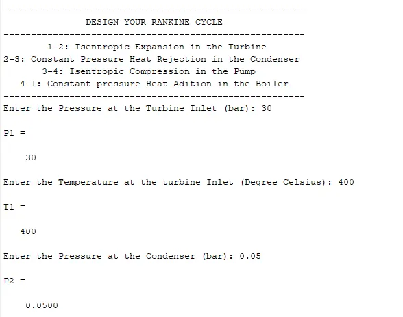
P1 = input('Enter the Pressure at the Turbine Inlet (bar): ')
T1 = input('Enter the Temperature at the turbine Inlet (Degree Celsius): ')
P2 = input('Enter the Pressure at the Condenser (bar): ')
% Solving the rankine cycle
% Creating the high pressure line
Tsat1 = XSteam('Tsat_p',P1);
Cpv1 = XSteam('CpV_p',P1);
Cpl1 = XSteam('CpL_p',P1);
Cpv4 = XSteam('CpV_p',P1);
Cpl4 = XSteam('CpL_p',P1);
% At Point 1'
hg1 = XSteam('hV_p',P1);
Sg1 = XSteam('SV_p',P1);
% At Point 4'
hf1 = XSteam('hL_p',P1);
Sf1 = XSteam('SL_p',P1);
% Creating the low presure line
Tsat2 = XSteam('Tsat_p',P2);
Cpv2 = XSteam('CpV_p',P2);
Cpl2 = XSteam('CpL_p',P2);
Cpv3 = XSteam('CpV_p',P2);
Cpl3 = XSteam('CpL_p',P2);
% At Point 2'
hg2 = XSteam('hV_p',P2);
Sg2 = XSteam('SV_p',P2);
% At Point 3
hf2 = XSteam('hL_p',P2);
Sf2 = XSteam('SL_p',P2);
% Calculating the state variables
% At Point 1
h1 = XSteam('h_pT',P1,T1);
S1 = XSteam('S_pT',P1,T1);
% At Point 2
S2 = S1;
if (S2 <= Sg2)
x2 = (S2-Sf2)/(Sg2-Sf2);
else
x2 = 1;
end
if (x2<1)
T2 = Tsat2;
h2 = hf2 + x2*(hg2-hf2);
else
% S = Sg2 + Cpv2*ln(T2+273/Tsat+273)
T2 = ((Tsat2+273)*exp((S2-Sg2)/Cpv2))-273;
h2 = hg2 + Cpv2*(T2-Tsat2);
end
% At Point 3 (No subcooling condition)
P3 = P2;
T3 = Tsat2;
h3 = hf2;
S3 = Sf2;
V3 = XSteam('vL_p',P3);
% At Point 4
P4 = P1;
S4 = S3;
Wp = (P4-P3)*V3*100;
% Wp = h4 - h3;
h4 = h3 + Wp;
% S4 = Sf1 + Cpl4*ln(T4/Tsat1)
T4 = (Tsat1*exp((S4-Sf1)/Cpl4));
Wt = h1 - h2;
Wnet = Wt - Wp;
Qin = h1 - h4;
Qout = h2 - h3;
Ntherm = Wnet/Qin;
SSC = 3600/Wt;
% Creating the saturation curve
T = linspace(1,T1,1000);
for i = 1:length(T)
hl(i) = XSteam('hL_T',T(i));
hv(i) = XSteam('hV_T',T(i));
Sl(i) = XSteam('SL_T',T(i));
Sv(i) = XSteam('SV_T',T(i));
end
% Getting the desired output
fprintf(' RESULTS \n')
fprintf('\n At State Point 1: \n')
fprintf('P1 = %f bar \n',P1)
fprintf('T1 = %f Degree Celsius \n',T1)
fprintf('h1 = %f kJ/kg \n',h1)
fprintf('S1 = %f kJ/kgK \n',S1)
fprintf('\n At State Point 2: \n')
fprintf('P2 = %f bar \n',P2)
fprintf('T2 = %f Degree Celsius \n',T2)
fprintf('h2 = %f kJ/kg \n',h2)
fprintf('S2 = %f kJ/kgK \n',S2)
fprintf('\n At State Point 3: \n')
fprintf('P3 = %f bar \n',P3)
fprintf('T3 = %f Degree Celsius \n',T3)
fprintf('h3 = %f kJ/kg \n',h3)
fprintf('S3 = %f kJ/kgK \n',S3)
fprintf('\n At State Point 4: \n')
fprintf('P4 = %f bar \n',P4)
fprintf('T4 = %f Degree Celsius \n',T4)
fprintf('h4 = %f kJ/kg \n',h4)
fprintf('S4 = %f kJ/kgK \n',S4)
fprintf('\n Other parameters: \n')
fprintf('Wt = %f kJ/kg \n',Wt)
fprintf('Wp = %f kJ/kg \n',Wp)
fprintf('Wnet = %f kJ/kg \n',Wnet)
fprintf('Ntherm = %f percent \n',Wp)
fprintf('S.S.C. = %f kg/kWhr \n',SSC)
% Plotting the graphs
figure(1)
hold on
plot(Sl,T,'linewidth',2, 'linestyle','--','color','b')
plot(Sv,T,'linewidth',2, 'linestyle','--','color','k')
plot([S1 S2],[T1 T2],'linewidth',1.5,'color','r')
plot([Sg2 S3],[Tsat2 T3],'linewidth',1.5,'color','g')
plot([S3 S4],[T3 T4],'linewidth',1.5,'color','c')
plot([Sf1 Sg1],[Tsat1 Tsat1],'linewidth',1.5,'color','m')
plot([S2 Sg2],[T2 Tsat2],[Sg2 S3],[Tsat2 T3],'linewidth',1.5,'color','g')
plot([S4 Sf1],[T4 Tsat1],'linewidth',1.5,'color','m');
plot([Sg1 S1],[Tsat1 T1],'linewidth',1.5,'color','m');
text(S1,T1,' 1');text(S2,T2,' 2');text(Sg2,Tsat2,' 2*');
text(S3,T3,'3 ','HorizontalAlignment','right','VerticalAlignment','bottom')
text(S4,T4,'4','HorizontalAlignment','right','VerticalAlignment','bottom')
text(Sf1,Tsat1,'4*','HorizontalAlignment','right','VerticalAlignment','bottom')
text(Sg1,Tsat1,' 1*')
xlabel('Entropy (kJ/kgK)')
ylabel('Temperature (Degree Celsius)')
title('T-S Diagram')
legend('Liquid curve','Vapour curve','Turbine','Condenser','Pump','Boiler')
grid on
hold off
figure(2)
hold on
plot(Sl,hl,'linewidth',2, 'linestyle','--','color','b')
plot(Sv,hv,'linewidth',2, 'linestyle','--','color','k')
plot([S1 S2],[h1 h2],'linewidth',1.5,'color','r')
plot([S2 S3],[h2 h3],'linewidth',1.5,'color','g')
plot([S3 S4],[h3 h4],'linewidth',1.5,'color','c')
plot([S4 S1],[h4 h1],'linewidth',1.5,'color','m')
text(S1,h1,' 1'); text(S2,h2,' 2')
text(S3,h3,'3','HorizontalAlignment','right','VerticalAlignment','top')
text(S4,h4,'4','HorizontalAlignment','right','VerticalAlignment','bottom')
xlabel('Entropy (kJ/kgK)')
ylabel('Enthalpy (kJ/kg)')
title('h-S Diagram')
legend('Liquid curve','Vapour curve','Turbine','Condenser','Pump','Boiler')
grid on
hold off
Results:
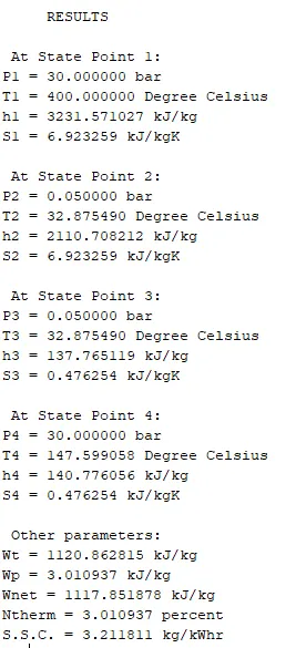
T-S Plot
h-S Plot
Errors:
No major errors faced while executing the MATLAB rpogram
Conclusion:
The required output values are obtained for the given output parameters:
- Net work output = 1117.87 kJ/kg
- Back work ratio = 0.003
Thus, the rankine cycle is simulated successfully using MATLAB.