Week 3 - External flow simulation over an Ahmed body.
Aim:
- The aerodynamics behaviour of the Ahmed body is numerically investigated using the Ansys fluent
- The body is perfectly symmetric; we can run the simulation by considering the only half body
- this is the best practice where we can save on the number of cells and get the results faster as well
Objective:
- To Describe Ahmed's body and its importance.
- To explain the reason for the negative pressure in the wake region.
- To explain the significance of the point of separation.
Abstract:
Ahmed body:
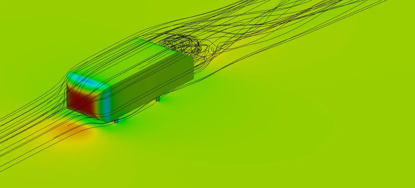
- The ahmed body is a simplified, generic vehicle model introduced by S.R.Ahmed in 1984 to study the aerodynamics behaviour of the ground vehicles.
- designed with a slanted rear surface, flat roof and sharp edges, it captures the essential features of flow separation, wake region and vortex strictures seen in real car aerodynamics, while avoiding the complexity of actual vehicle geometries.
- widely used in both experimental and CFD research, the ahmed body serves as a benchmark case for validating turbulence models and analyzing drag characteristics.
- Its aerodynamics performance, especially the drag co-efficient is strongly influenced by the rear slant angle, making it a valuable tool in automotive design and aerodynamic optimization studies.
- the particular goal of this benchmark is to compare the drag coefficient, velocity profiles, velocity field and time average wake structure of the ansys simulation results with the real experimental measurements in the wind tunnel
Modelling approach:
- In this simulation we analyze the turbulent flow around an ahmed body using the K-epsilon turbulence model.
- This flow is classified as turbulent because the Re exceeds 2000, indicating a fully developed turbulent regime.
- The K - epsilon model is well suited for high reynolds number flows that are steady and nearly in equilibirum, especially where large pressure gradients are not dominant.
- This model approximates the behaviour of turbulence without explicitly resolving the viscous sublayer near walls, making it computationally efficient for external aerodynamics appications.
- The ahmed body used in this study is a simplifed geometric representation of a ground vehicle.
- Though geometrically simple, it captures essential aerodynamic characteristics relevant to real world automotive designs, such as flow separation and wake formations.
- It uses allows for a balance between simulation accuracy and computational manageability.
- The objective of this setup is to simulate and analyze the turbulent flow field around the ahmed body and validate the results using the turbulent flow, K-epsilon approach within a CFD framework.
2D Geometry of Ahmed body:
- This model is performed as a similitude study where it is an art of predicting prototype performing from model observation
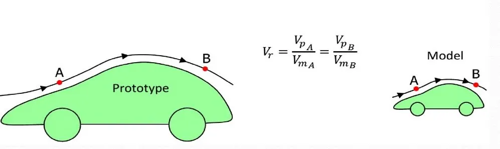
- where ahmed body is a model and roughly it is scaled as 1:4 of compact automotive passenger vehicles
- It simplifies complex features (wheels, mirrors, curved surfaces into clean geometric surface to isolate aerodynamic behaviour like boundary layer development, flow separation at rest slant, wake and vortex formation.
Key features dimensions:
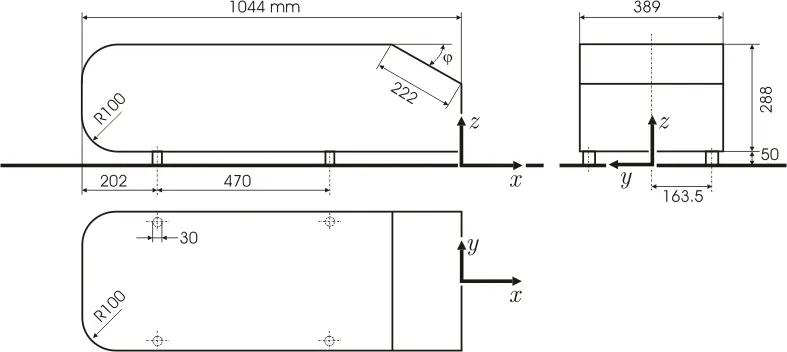
Overall length - 1044 mm
Overall height - 288 mm
Width - 389 mm
Wheelbase equivalent - 470 mm
Ground clearance - 50 mm
Rear slant Length - 222 mm with an angle of 30 degree
Round front Radius - R100 mm
- so, the rear body slant angles are the important parameter for this analysis as it gives the aerodynamic parameters which is important for analyzing the drag co-efficient.
Solution approach:
Step 1: Geometry creation:
- The ahmed model step file is imported in ansys geometry tab and edited using ansys space claim. the dimensions are same as we seen above.
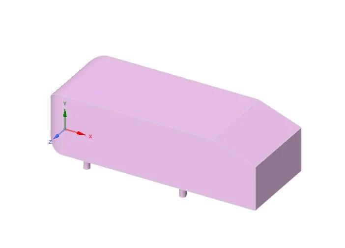
- so here, we need to run the external flow aerodynamic simulation by mic the physical wind tunnel experiment in labs.
- therefore, we will be creating the external boundary for the ahmed body using enclosure option.
- there will be two layers of enclose will be used in this problem
- An enclosure is a defined fluid domain that surrounds a physical model, providing sufficient space for flow development and minimizing boundary effects.
- In this case, a box-shaped enclosure has been created around the Ahmed body.
- The dimensions of the outer enclosure are set to ensure proper flow capture: it extends 2 meters upstream from the front of the Ahmed body, 5 meters downstream from the rear, 1 meter above the top surface, and 0 meters below (ground clearance). On the lateral sides, a clearance of 0.5 meters is maintained on both ends to accommodate lateral flow behavior.
- To improve computational efficiency and better resolve critical flow regions—especially near the walls and wake zone—an inner enclosure is added within the outer domain.
- This refined enclosure is designed based on observations from a baseline simulation.
- It extends 0.5 meters upstream from the front of the body, 1 meter downstream from the rear, 0.5 meters above the top surface, and also starts from ground level. This dual-enclosure strategy ensures accurate flow capture where needed while optimizing mesh density and simulation runtime.
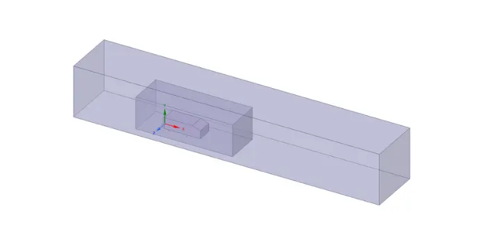
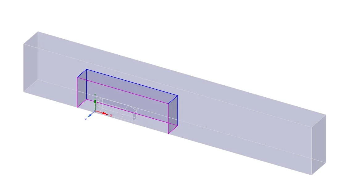
- As the body is perfectly symmetric, we can run the simulation by considering the only half body.
- This is the best practice where you can save on the number of cells and get the results faster as well
- after spliting the body, we need to give the share topology for the two enclosures. which will help to share the information throughout the cells
Step 2: Meshing:
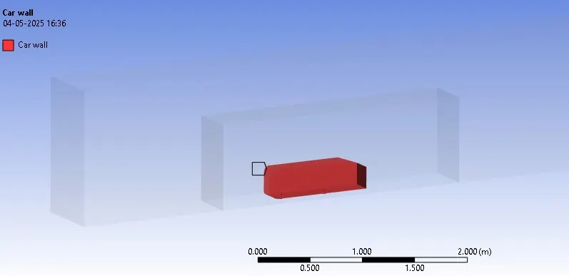
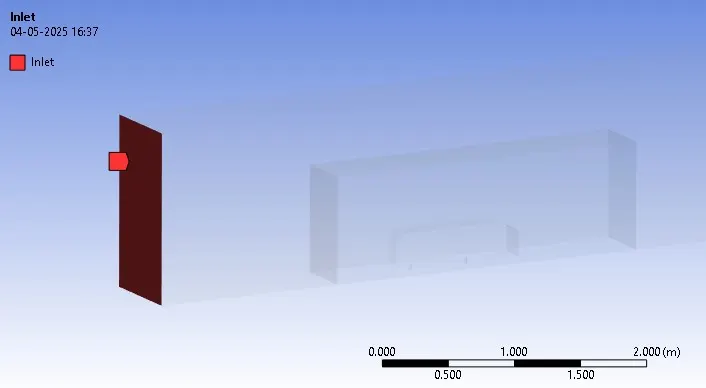
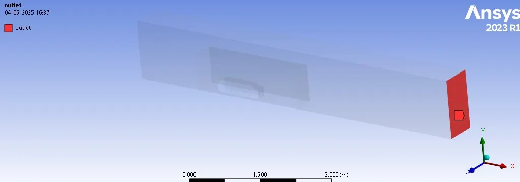
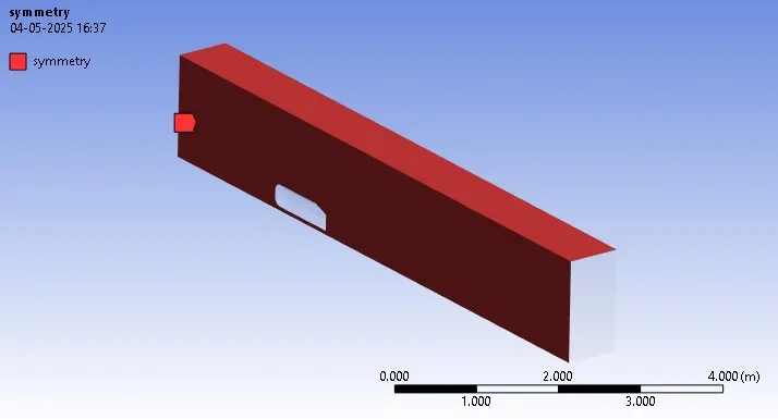
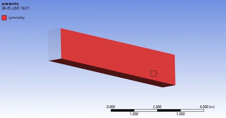
before starting with mesh generation, we need to give the name selection for each corresponding faces which is used for this simulation
1) car wall
2) inlet
3) outlet
4)symmetry faces
- After that we create first the baseline mesh of element size is 100mm and generate the mesh for the hexahedral we have to go insert sizing and select the multizone for the different mesh patterns. It will generate hexahedral baseline automatically because hexahedral meshes are more accurate that tetrahedral meshes.
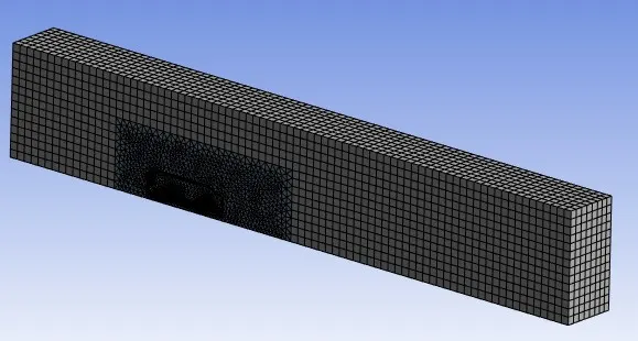
- For the local refinement region mesh size we are using it 50mm for because the as the mesh is much finer the more accurate the result It will captures the flow behaviour at every point. Right click on the mesh go to insert option and then select the sizing option. Select the inner box then give the element size 50mm and generate mesh.
Here we have the important parameter in this analysis - Y+
To describe the fluid flow near walls, two dimensionless quantities, U+ and Y+ are used. these are defined as follows
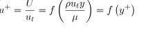
- This equation is called as law of the wall.
- U is the velocity (m/s) at distance y from wall,
- UT is the friction velocity (m/s),
- ρ is the density of the fluid (kg/m3)
- μ is the viscosity (pa.s)
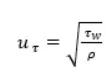 , the friction velocity
Tw is the wall shear stress
Generally, different Y+ ranges are used for different purposes
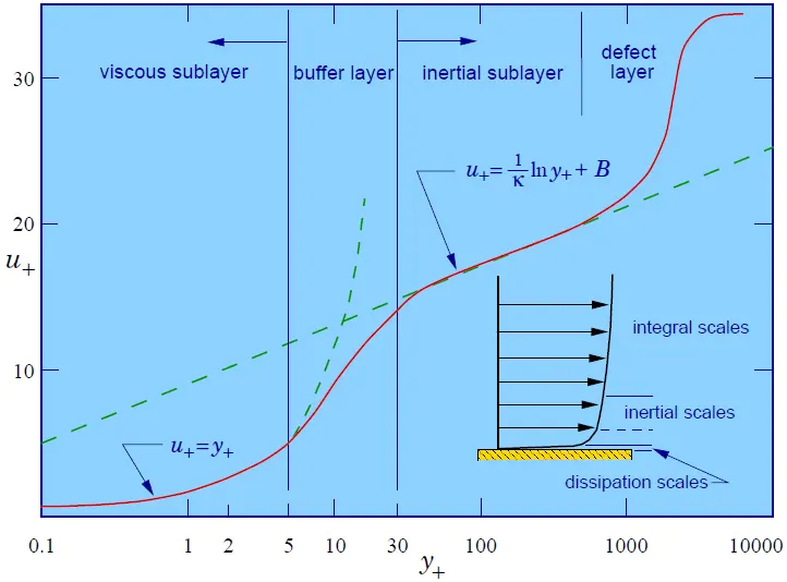
Linear or viscous sub layer (Y+ < 5):
- In this region very close to the wall, the fluid velocity is very low, and viscous force is completely dominant.
- That is why is called the viscous sub-layer.
- It is assumed that the shear stress is approximately constant and equal to the wall shear stress.
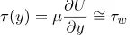
- after intergrating with respect to y and applying the boundary conditions U = 0 and Y = 0, we obtain a linear relationship between the mean velocity and the distance from the wall

- by performing some algebraic operations and using the definition of U+ and Y+, we obtain
U+ = Y+
- because of the linear relationship between U+ and y+. this area is known as the linear sub layer.
Buffer layer (5 < y+ < 30)
- This layer is between the layer of the viscous sublayer where the viscous force is dominant and the log law layer where the inertial force is dominant.
- In this layer, neither the inertia force nor the viscous force is dominant and both are effective.
- Therefore, the speed distribution in this layer is different from the previous and next layers.
- CFD simulation software address the buffer layer by utilizing a combination of mesh refinement, turbulence modeling and near wall treatment strategies.
- some turbulent flow simulation model such as low Re number models or hybrid approaches are usually used to calculate the flow distribution in the complex buffer layer area.
- these turbulence model usually use damping function or blending techniques to calculate velocity changes from the viscous sublayer to log law layer.
Log law layer (30 <Y+ <500)
- In this layer, both viscous and turbulent effects are important. the velocity distribution is
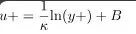
- von karman's constant (k) is approximately 0.4 and B is and empirical constant, typically around 5.5
Why should Y+ be calculated in CFD
- depends on which turbulence model you use and what your simulation goal is, your mesh resolution in the neighborhood of the wall need to have different sizes.
- before simulation, calculate the y+ value for CFD simulation using problem parameters.
- then use tow methods to determine the resolution of the mesh next to the wall
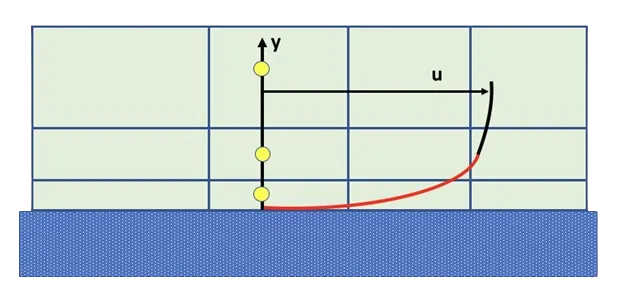
Wall function approach:
- Compared to other method, this method has a coarser mesh, which reduces its computational expense.
- for complex flows with flow separation or high-pressure gradients, this method is less accurate.
- It is recommended to use this method, the center of the first mesh cell should be at 30< y+ < 300.
Near wall model approach (Low reynolds number modelling):
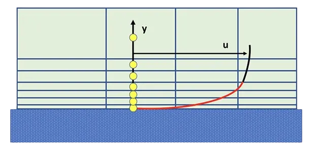
- In this method, the viscous sublayer is simulated with a fine mesh in the area next to the wall where the viscous force is dominant.
- This method provides proper accuracy in simulating complex flows and flow separation.
- To achieve high accuracy results, this method required Y+ values of approximately 1 or less.
- Although this method has high accuracy, it requires high computing power due to the small mesh.
- This method is recommended when your goal is to measure forces on walls.
- The standard K-epsilon model is recommended for simulating free stream flows, but it is incapable of simulating the flow around the walls
- so, in this turbulence model, wall function is usually used for calculating near the walls.
- On the other hand, K omega SST model is known for its ability to simulate flows around the walls
For this project Y+ calculation:
Fluid - air
Fluid temperature - 25 degree C
Free stream velocity - 25 m/s
Domain length (ahmed body) - 1.044 m
density of air - 1.184 kg/m3
dynamic viscosity of air - 1.849 x 10⁻⁵ kg/ (m.s)
kinematic viscosity of air - 1.562 x 10⁻⁵ m2/s
Reynold number:
Re = (ρ*U*L) / μ
Re = (1.184 * 25 * 1.044) / 1.849 x 10⁻⁵
Re = 1671303
Skin co-efficient using blasius formula
Cf = 0.026/ Re(1/7)
Cf = 0.026/1671303(1/7)
Cf = 0.003357
Wall shear stress
Tw = 1/2*Cf*ρ*U2
Tw = 1/2 * 0.003357 * 1.184 * 252
Tw = 1.24209 Pa
Friction velocity
Ut = √(Tw/ρ)
Ut = √(1.24209/1.184)
Ut = 1.02423 m/s
Here are the three case of Y+ which will be calculated
Case 1: Y+ = 50 (fine mesh)
Case 2: Y+ = 150 (moderate mesh)
Case 3: Y+ = 290 (coarse mesh)
Case 4: Y+ = 1 (very fine mesh)
Case 1:
Y = (ν * Y+)/Ut
Y = (1.562 x 10-5* 50)/1.02423
Y = 0.000740 m
Here, we calculate the total thickness on the basis of first cell height (Y) we got from the assumed Y+ value.
Y+ value tells where mesh lies So, the total thickness of the inflation layer is
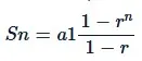
a1 = first term of first layer of thickness
r = growth rate
n = no. of layers
Sn = 0.7 [(1 - 1.26)/ (1 - 1.2)]
Sn = 6.95 mm
Case 2:
Y = (ν * Y+)/Ut
Y = (1.562 x 10-5* 150)/1.02423
Y = 0.00228 m
Sn = 2.28 [(1 - 1.26)/ (1 - 1.2)]
Sn = 22.640 mm
Case 3:
Y = (ν * Y+)/Ut
Y = (1.562 x 10-5* 290)/1.02423
Y = 0.00442 m
Sn = 4.42 [(1 - 1.26)/ (1 - 1.2)]
Sn = 43.890 mm
Case 4:
Y = (ν * Y+)/Ut
Y = (1.562 x 10-5* 290)/1.02423
Y = 0.0000152 m
Sn = 0.0152 [(1 - 1.26)/ (1 - 1.2)]
Sn = 0.150 mm
This inflation layer will vary upon each case
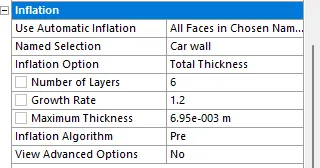
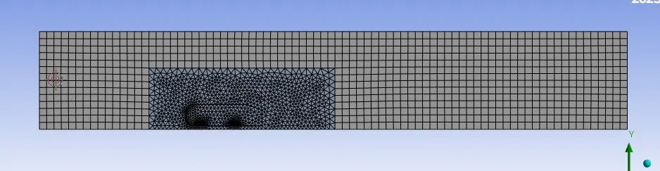
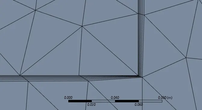
Inflation layer in car walls
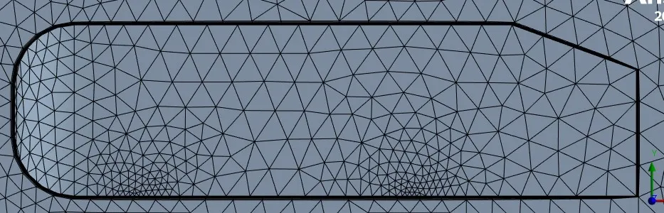
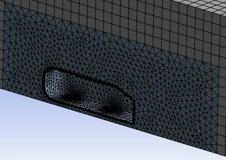
Further zoom in, we can see the inflation layer which is for case 1. hence it is small
Step 3: Analysis setup:
For case 1, 2 and 3 we are using K-epsilon standard and case 4 uses K-omega SST viscous model.
Reference values (air at 25-degree Celsius)
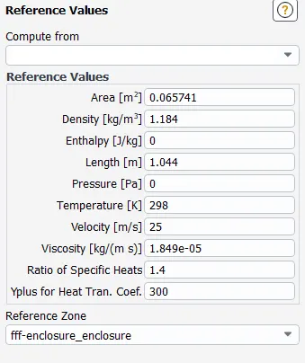
- area is taken here is frontal area of the ahmed body
- Length is the ahmed body length in m
- energy equation is used here, to capture the temperature domain also
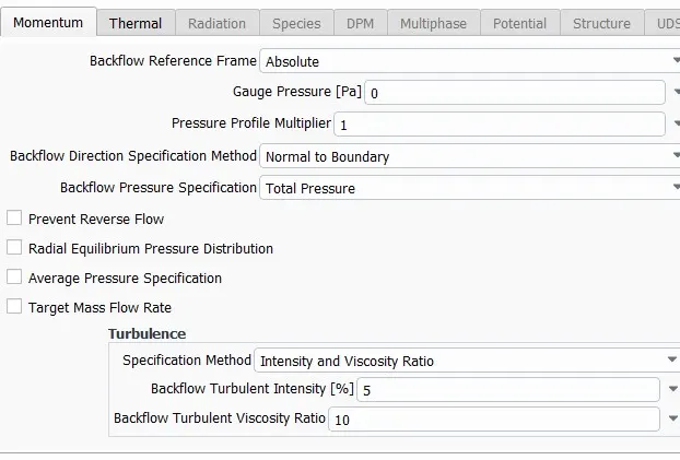
Boundary conditions
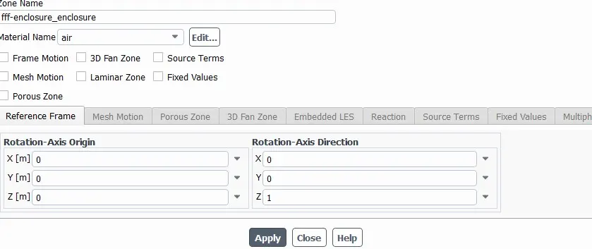
In cell zones, the material type is given as fluid which is air at 298K
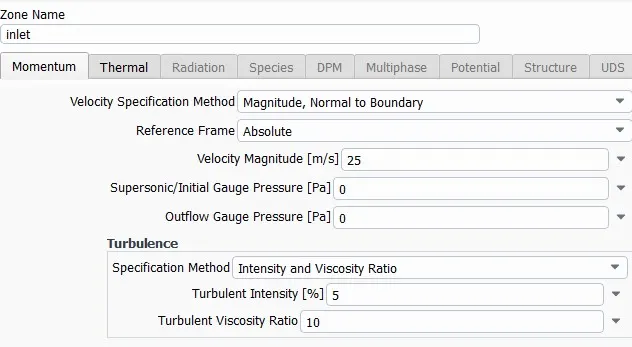
- Inlet velocity is 25 m/s at a temperature of 298K
- Outlet pressure will be gauge pressure
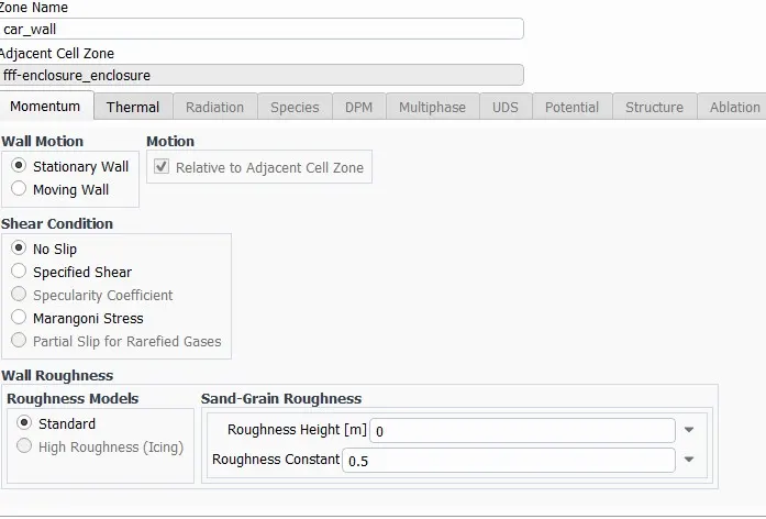
- car wall is automatically taken as wall type
- In solution initialization we use Hybrid, where method Fluent uses to generate an initial guess for the flow field before solving begins. It works by solving simplified equations (not the full Navier-Stokes) to create a physically reasonable starting solution — better than just assuming everything starts from zero.
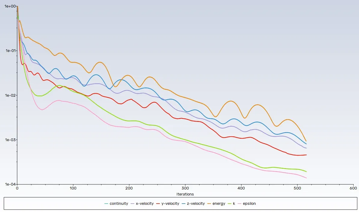
- Then define the residual plot which are required for this analysis.
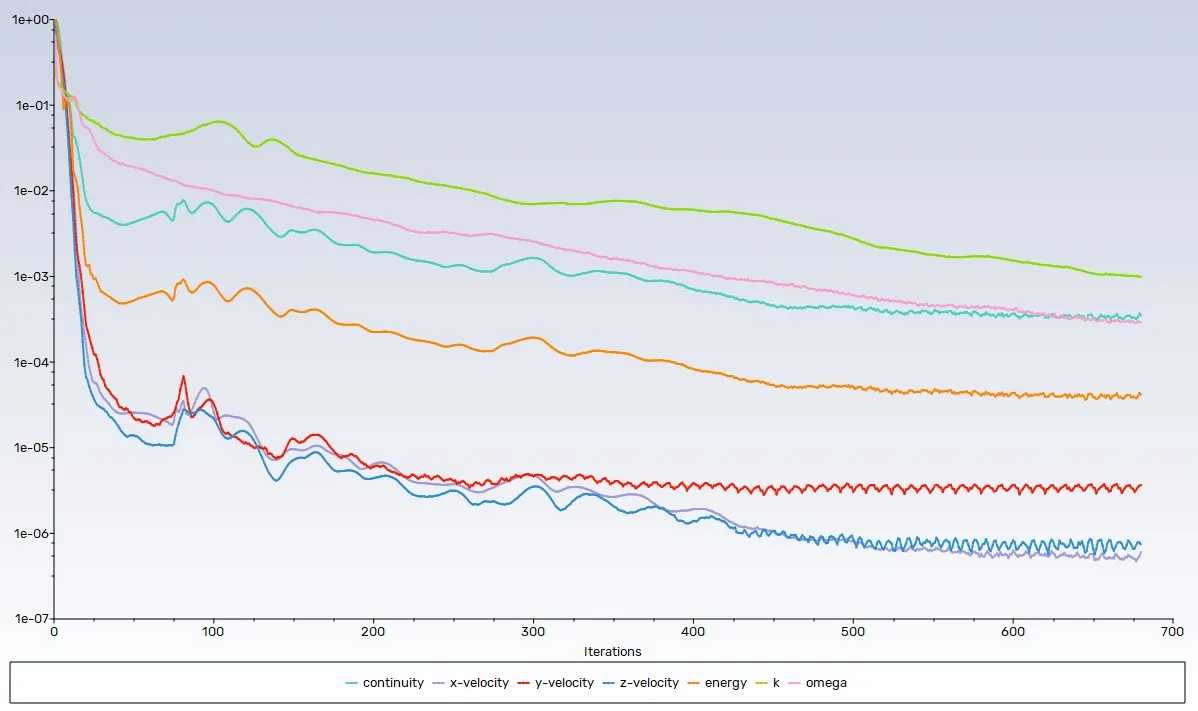
- Then solution is kept run untill it gets converged.
Setup 4: solution report
Case 1: y+ 50 (k-epsilon standard)
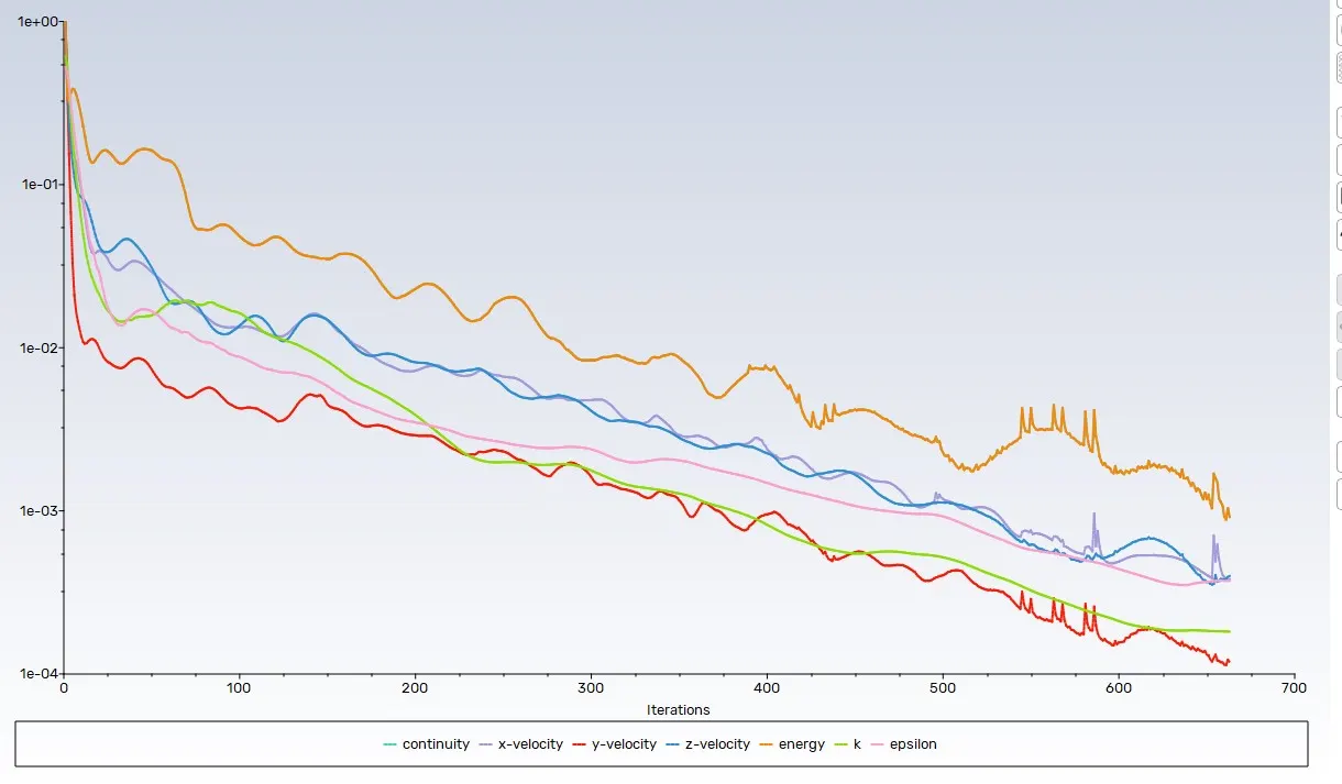
Residual plot:
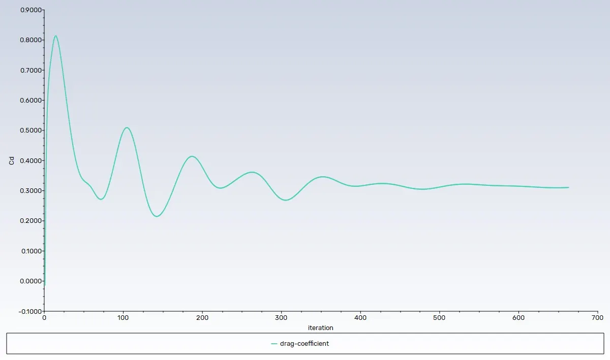
Drag co-efficient plot:
Lift co-efficient plot:
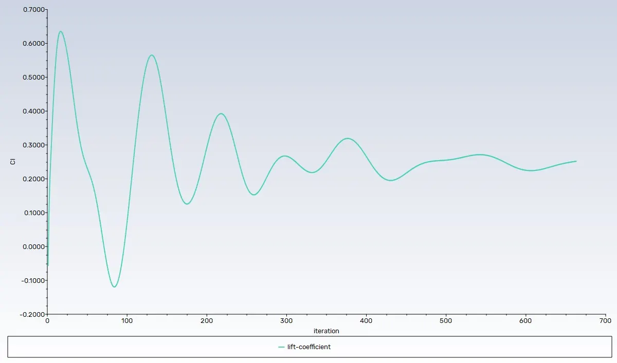
Convergence:

Velocity vector contour:
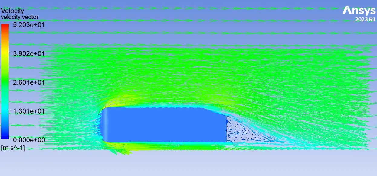
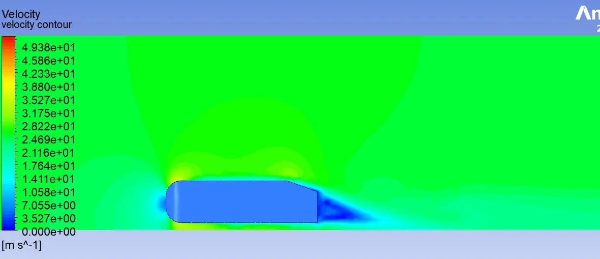
Streamline velocity:
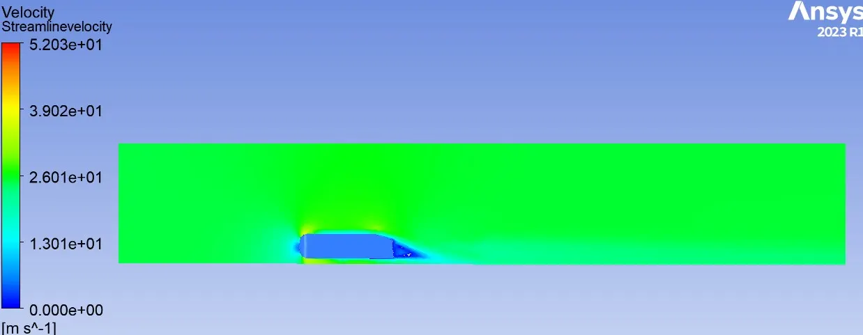
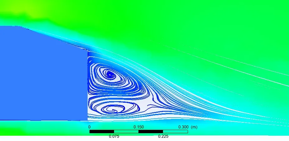
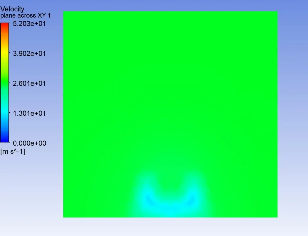
Velocity contour across XY plane (wake region)
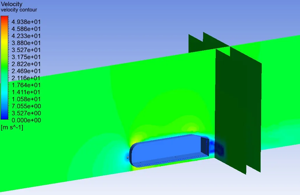
X - 0.106 m from back of the car
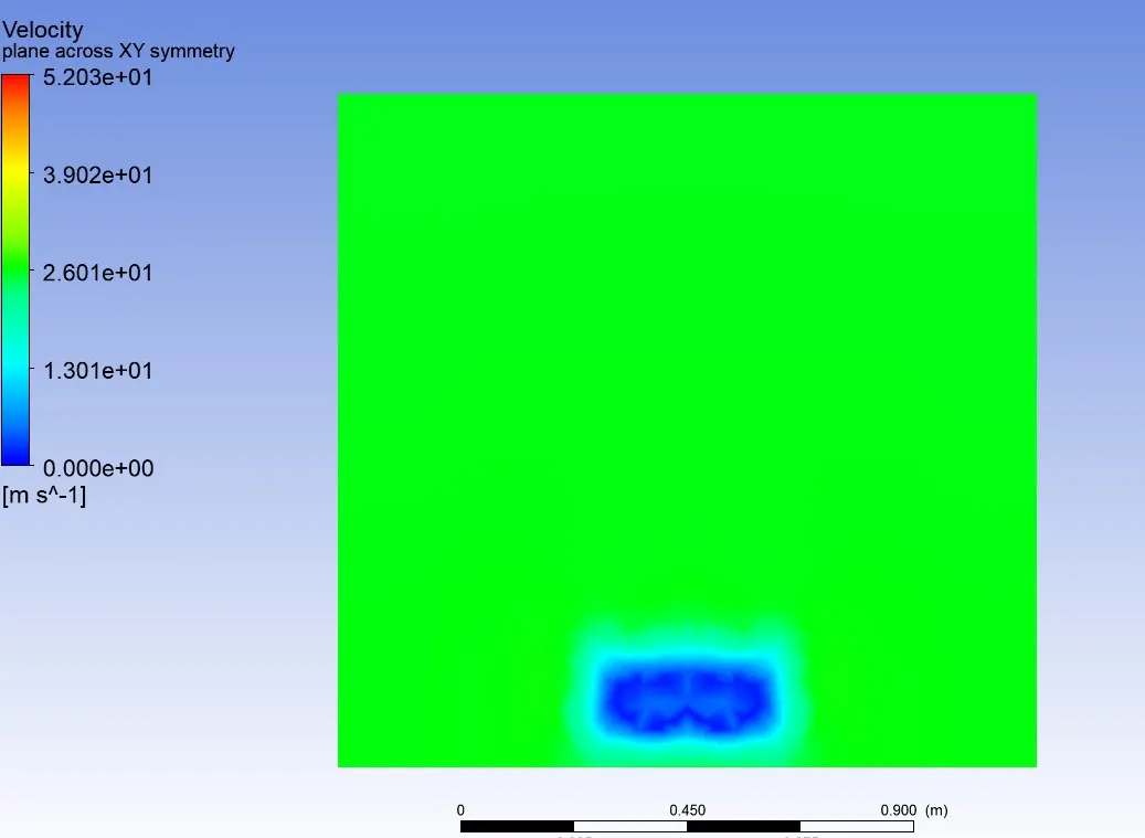
X - 0.300 m from back of the car
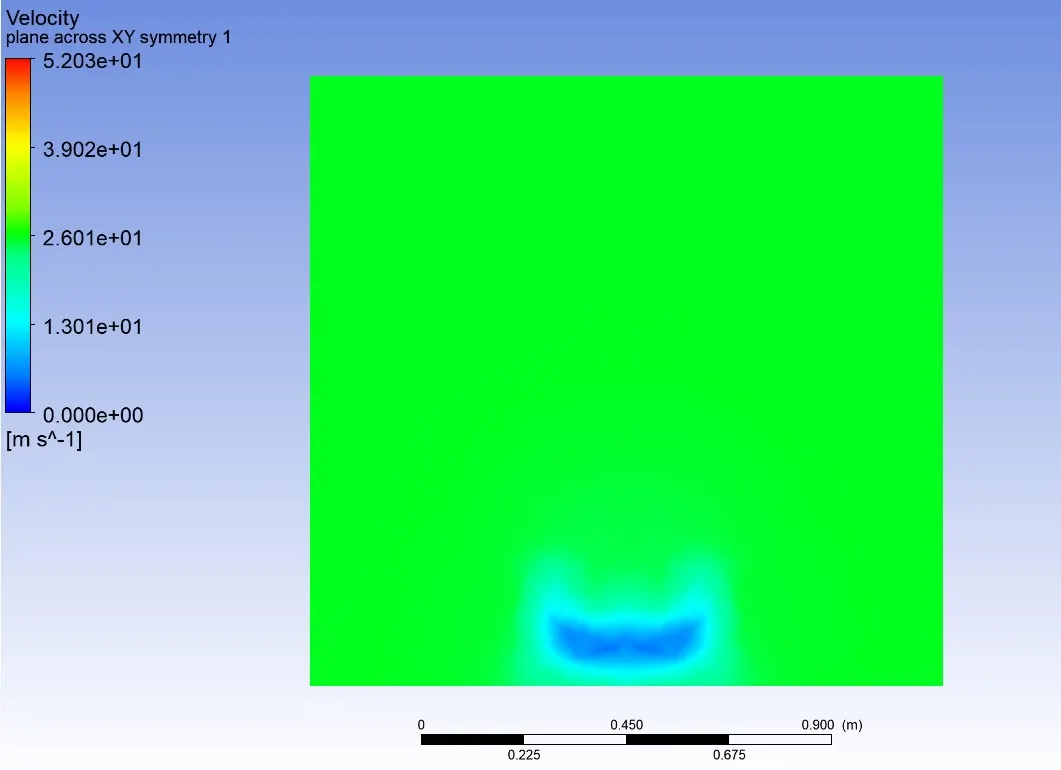
X - 0.450 m from back of the car
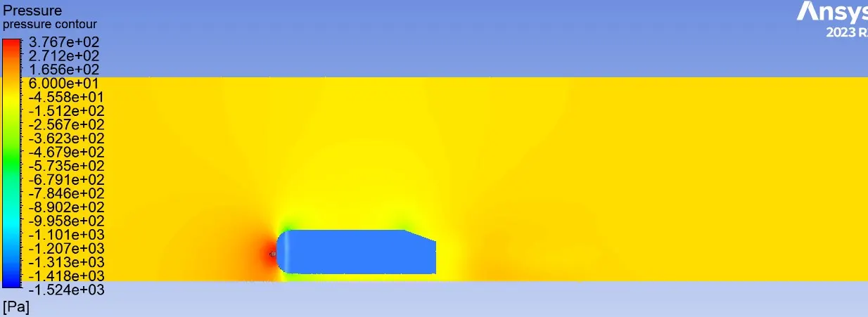
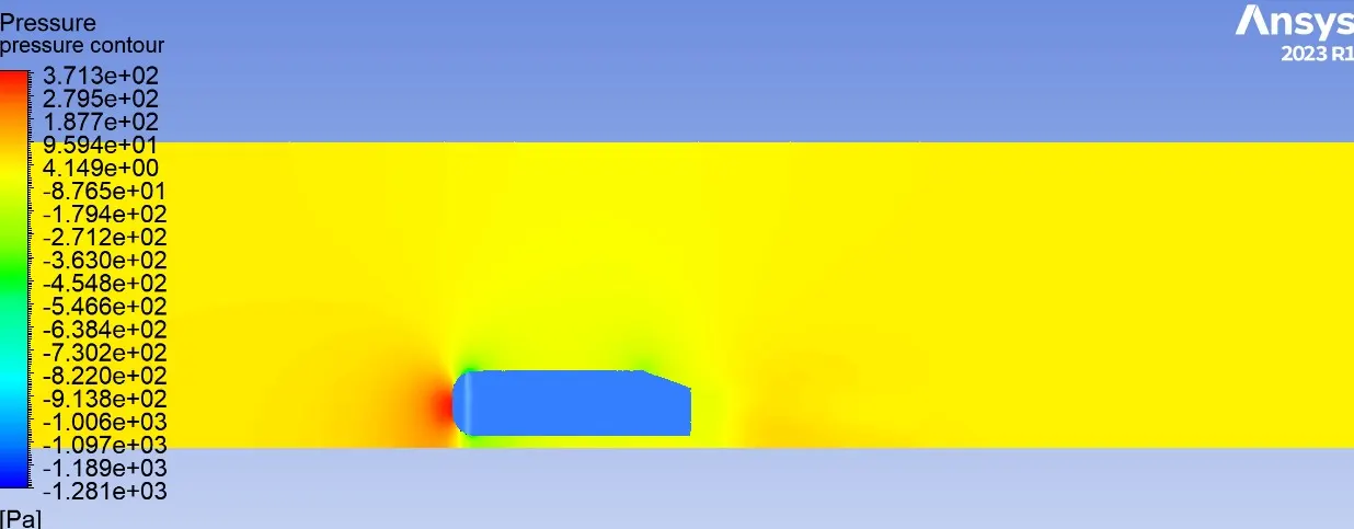
Pressure contour along XY plane:
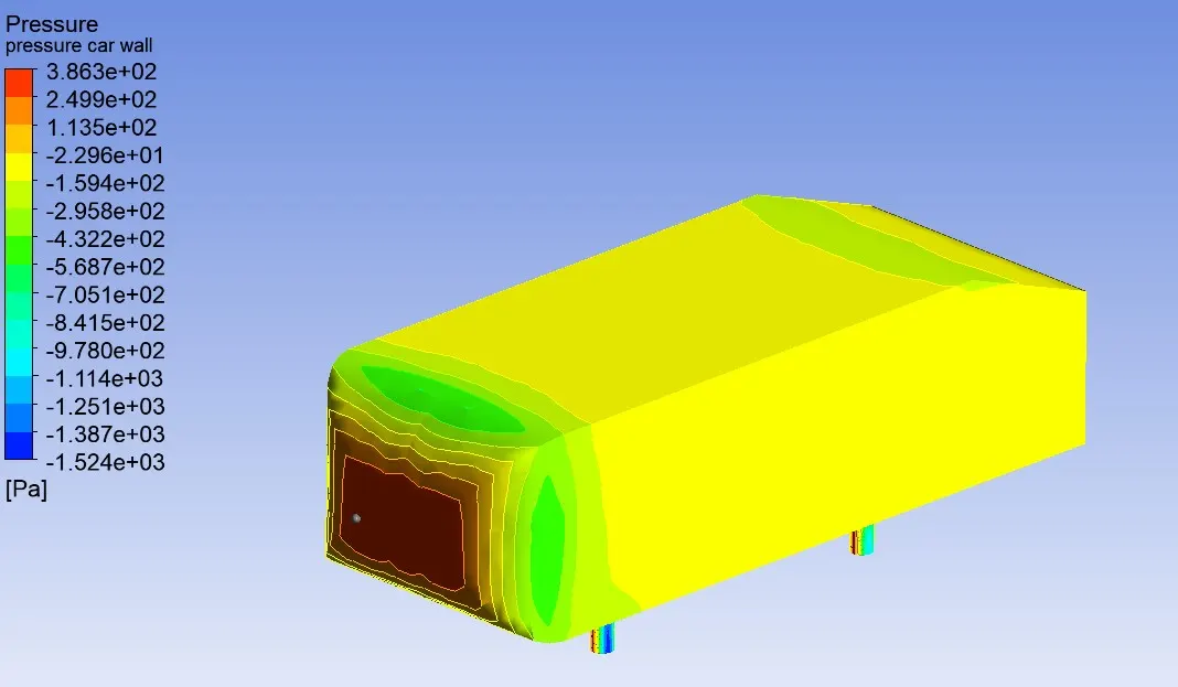
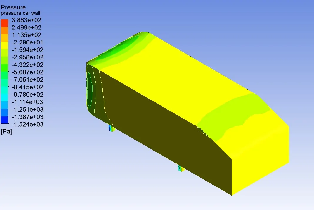
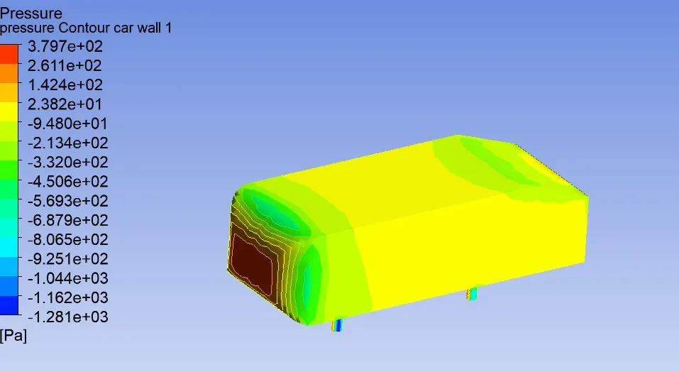
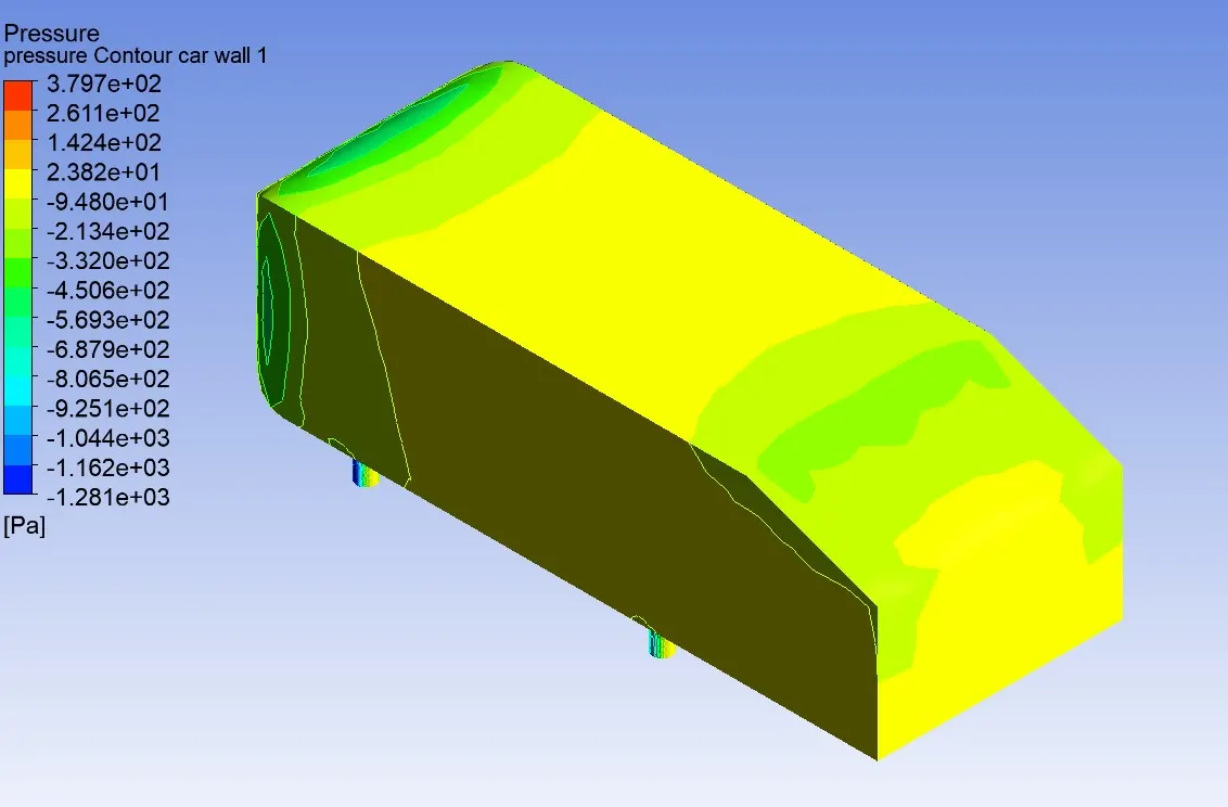
Pressure contour in car wall:
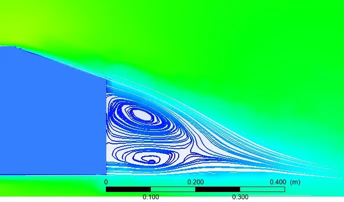
Case 2: y+ 150 (k-epsilon standard)
Residual plot:
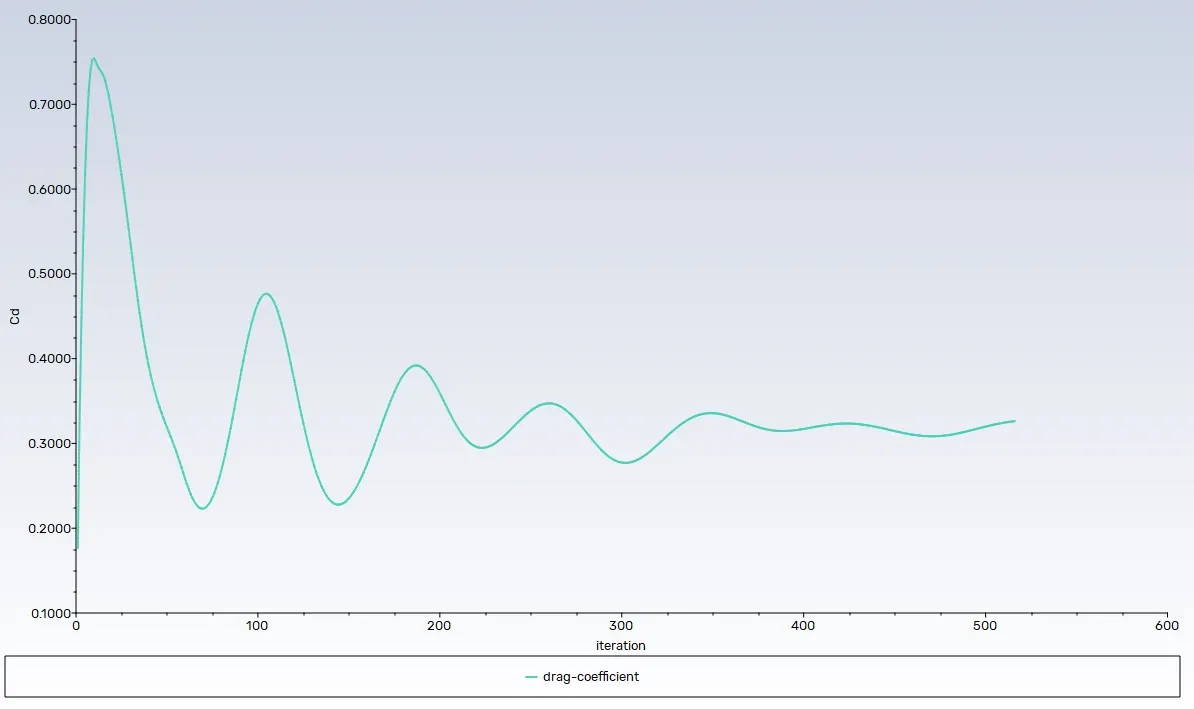
Drag co-efficient plot:
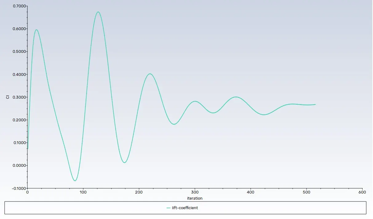
Lift co-efficient plot:
Convergence:

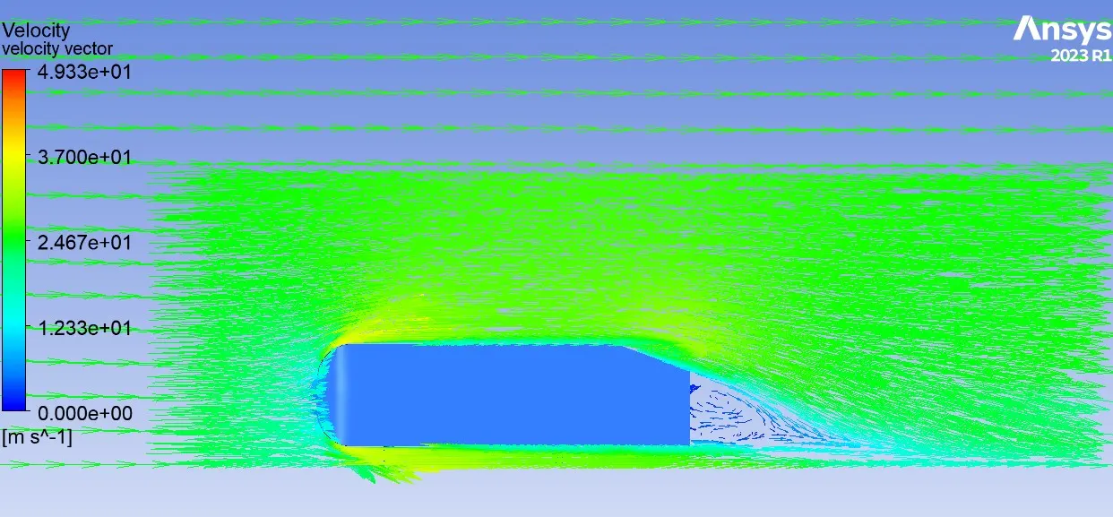
Velocity vector contour:
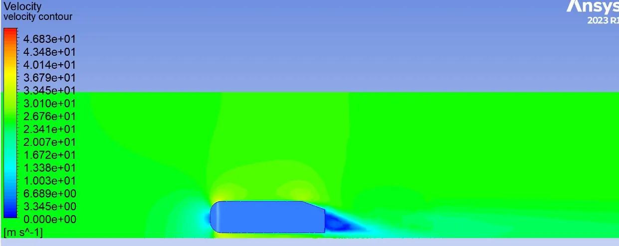
Streamline velocity:
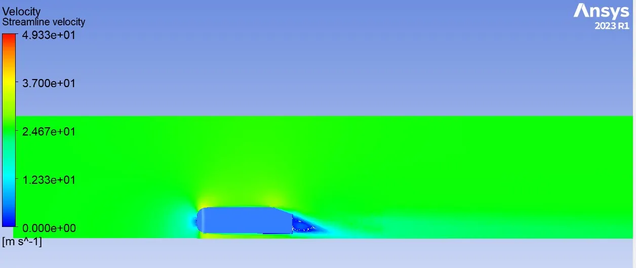
Velocity contour across XY plane (wake region)
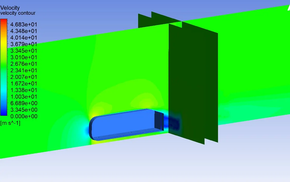
X - 0.106 m from back of the car
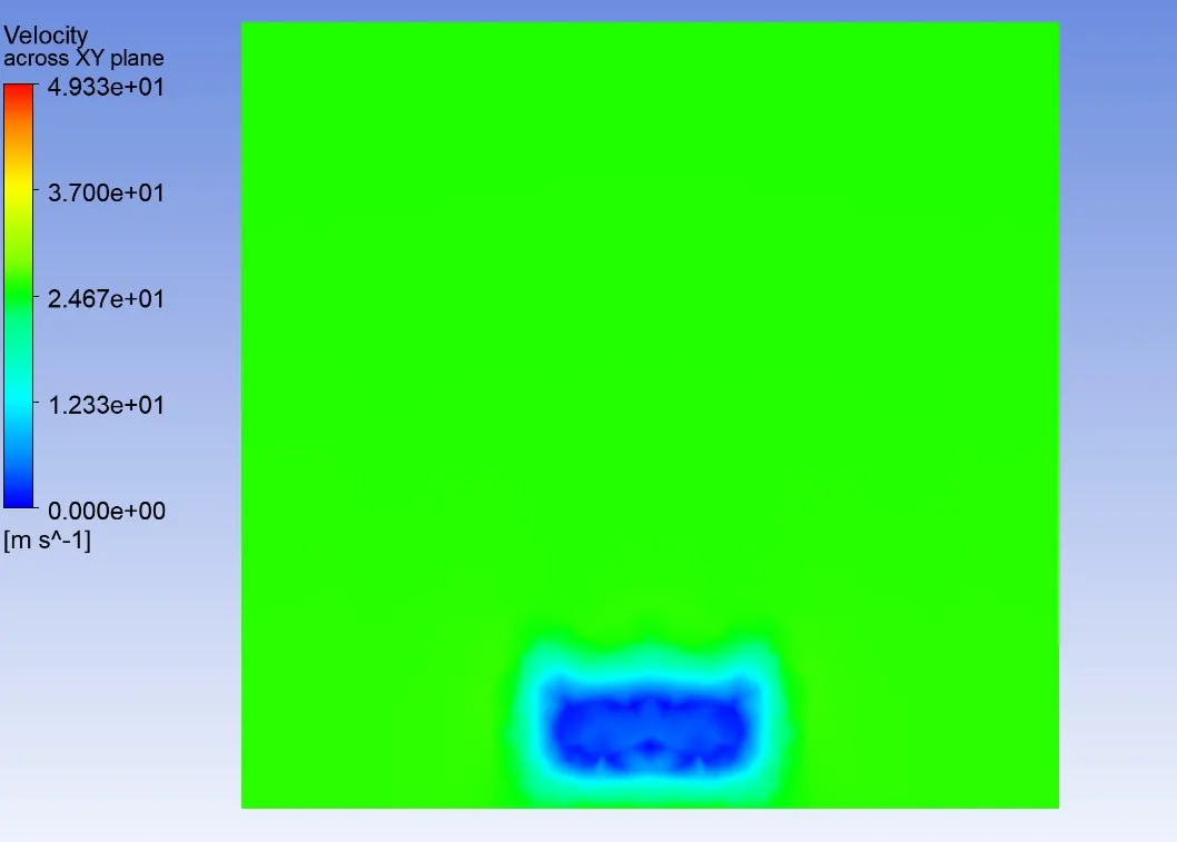
X - 0.300 m from back of the car
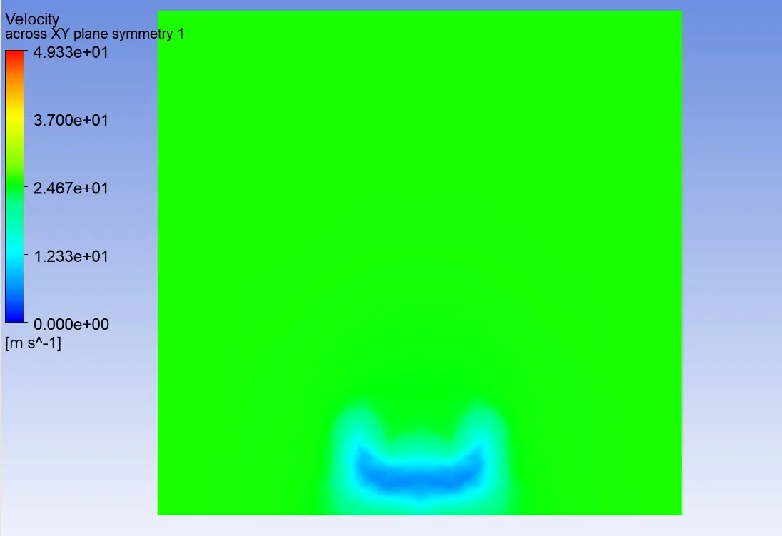
X - 0.450 m from back of the car
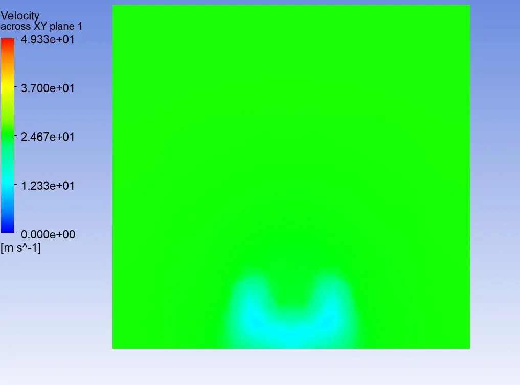
Pressure contour along XY plane:
Pressure contour in car wall:
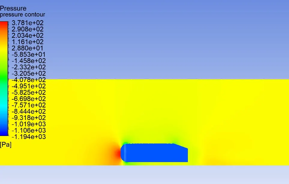
Case 3: y+ 290 (k-epsilon standard)
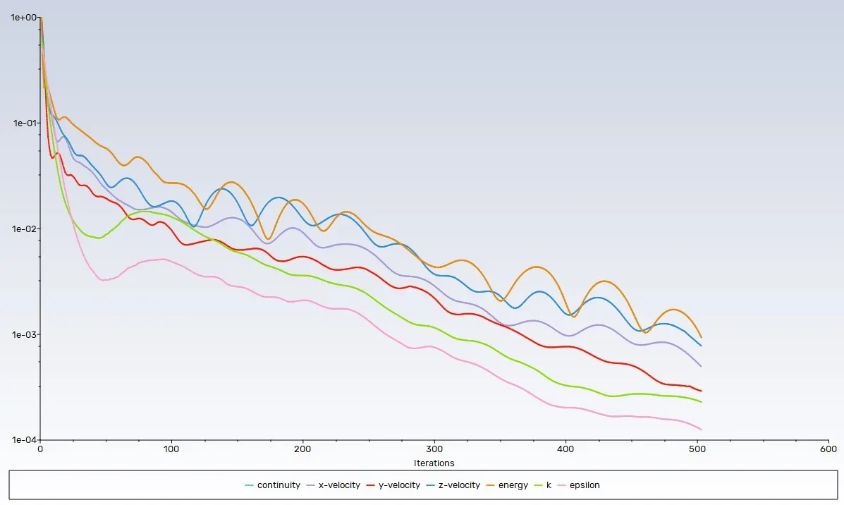
Residual plot:
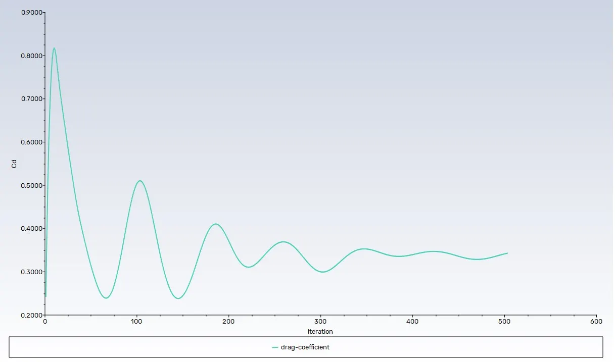
Drag co-efficient plot:
Lift co-efficient plot:
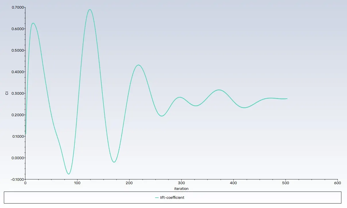
Convergence:

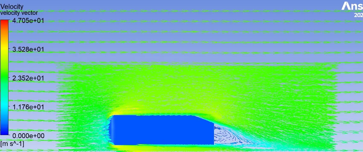
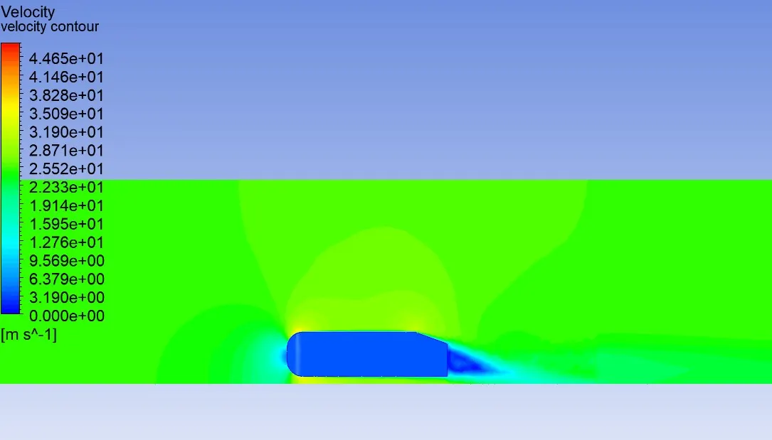
Velocity vector contour:
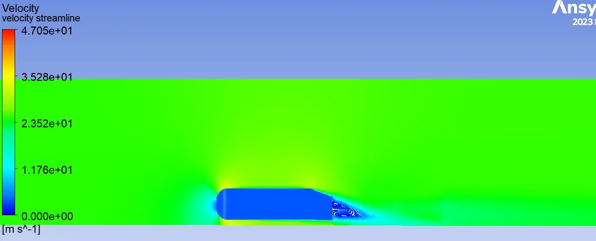
Streamline velocity:
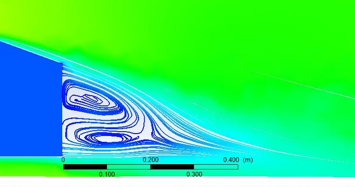
Velocity contour across XY plane (wake region)
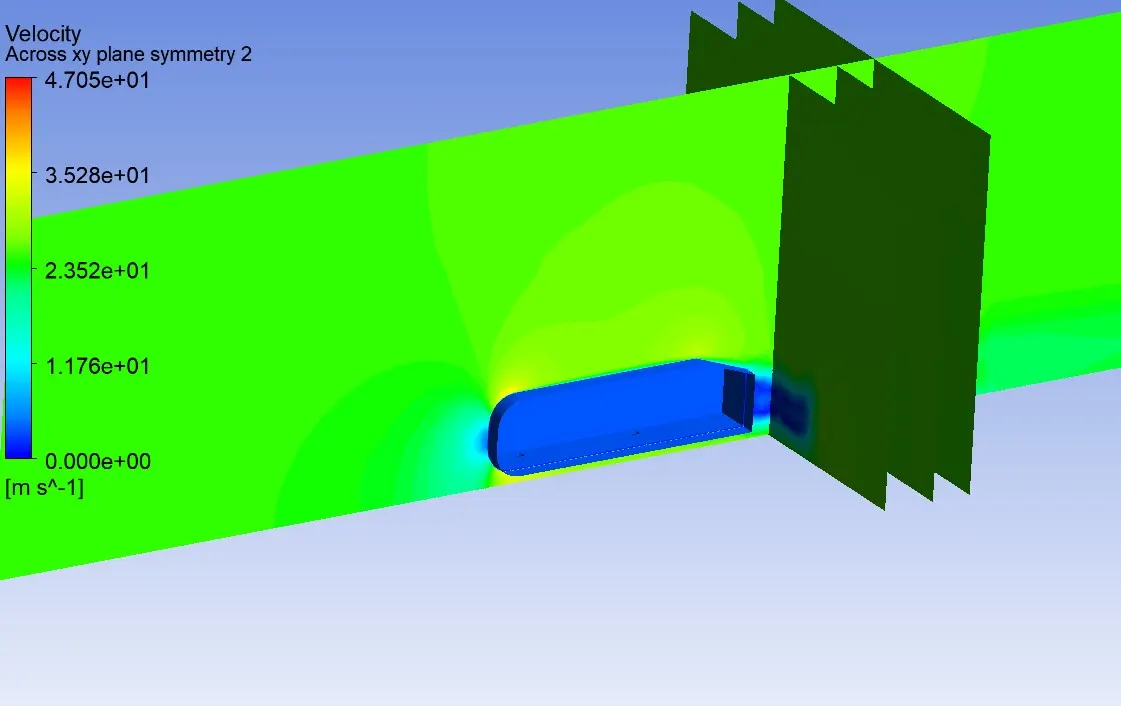
X - 0.106 m from back of the car
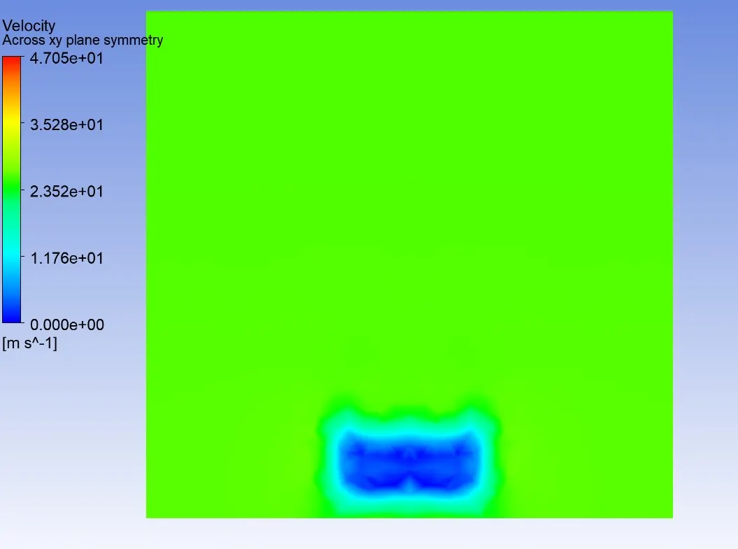
X - 0.300 m from back of the car
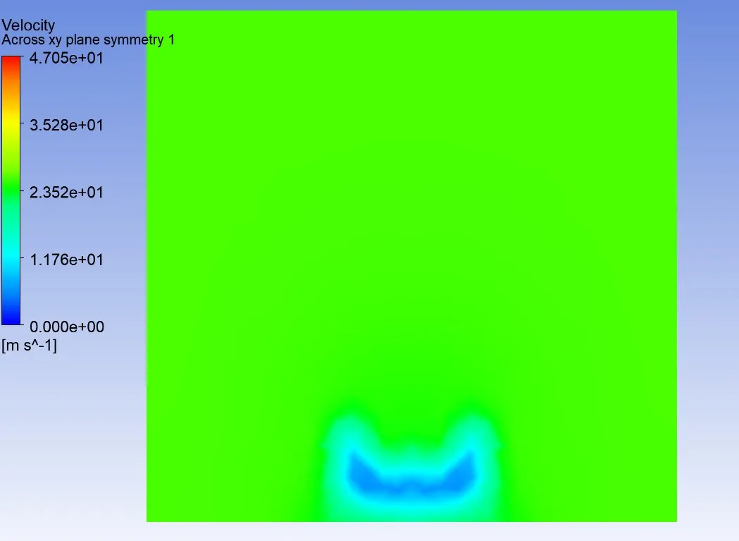
X - 0.450 m from back of the car
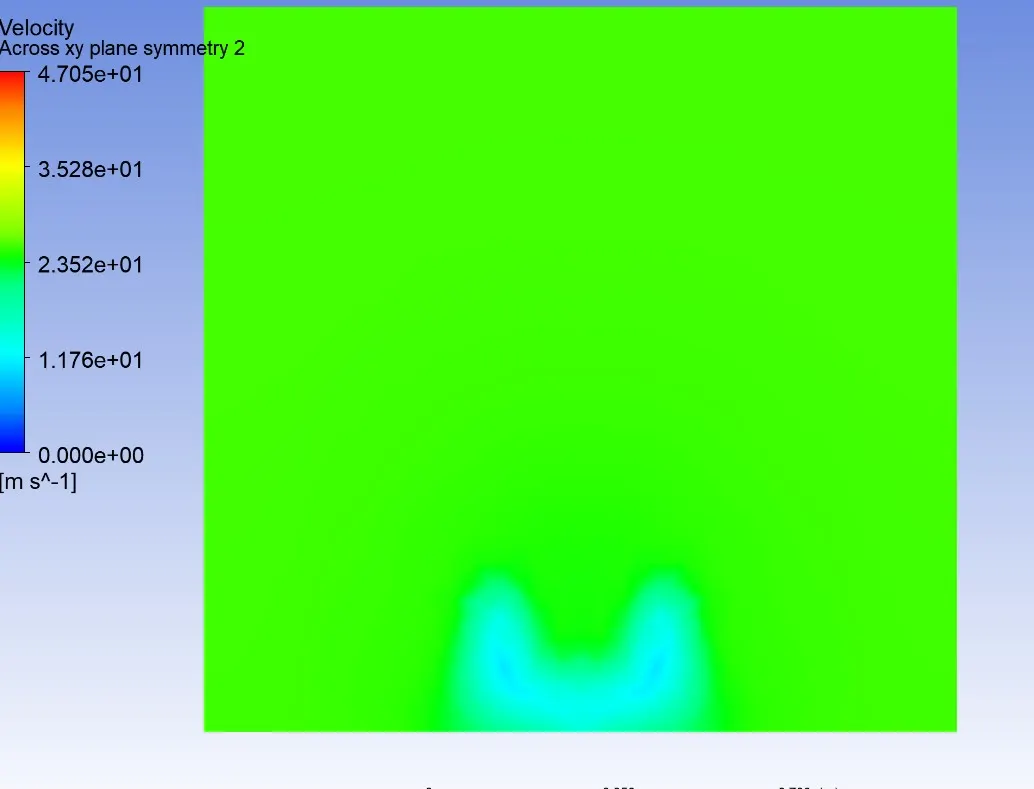
Pressure contour along XY plane:
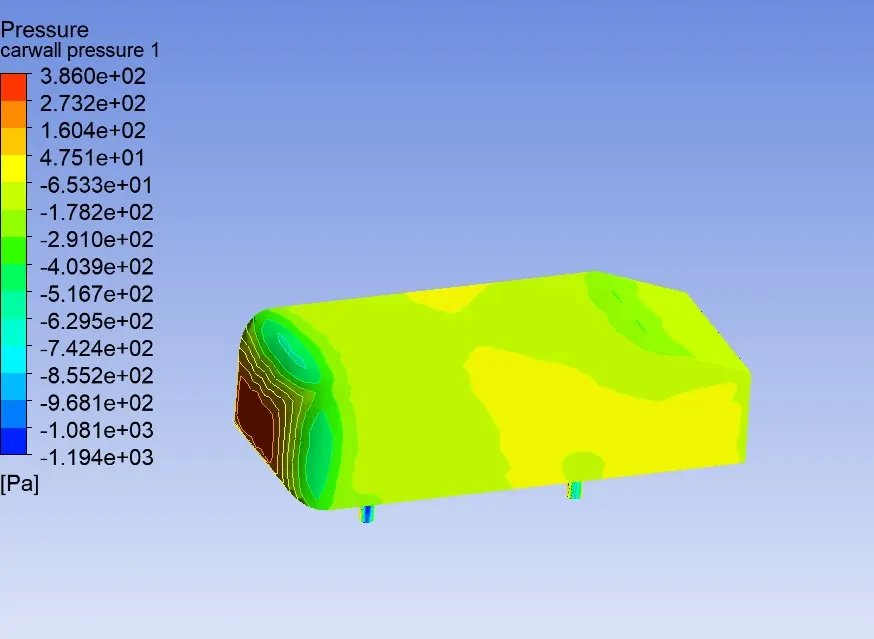
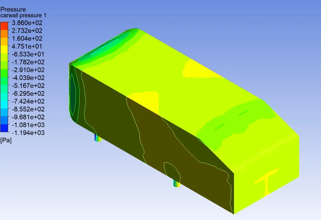
Pressure contour in car wall:
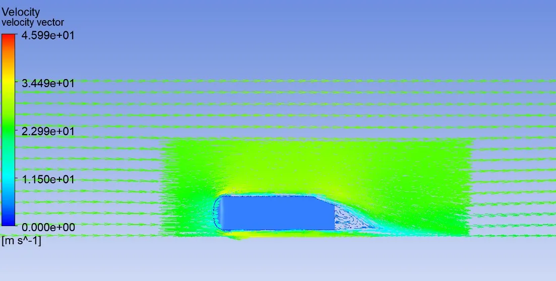
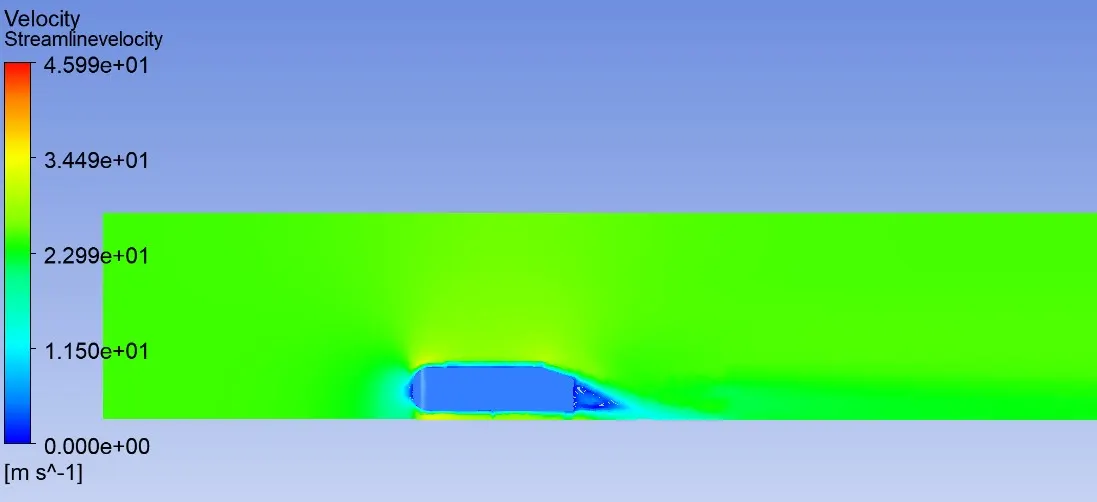
Case 4: y+ 1 (k-Omega SST)
Residual plot:
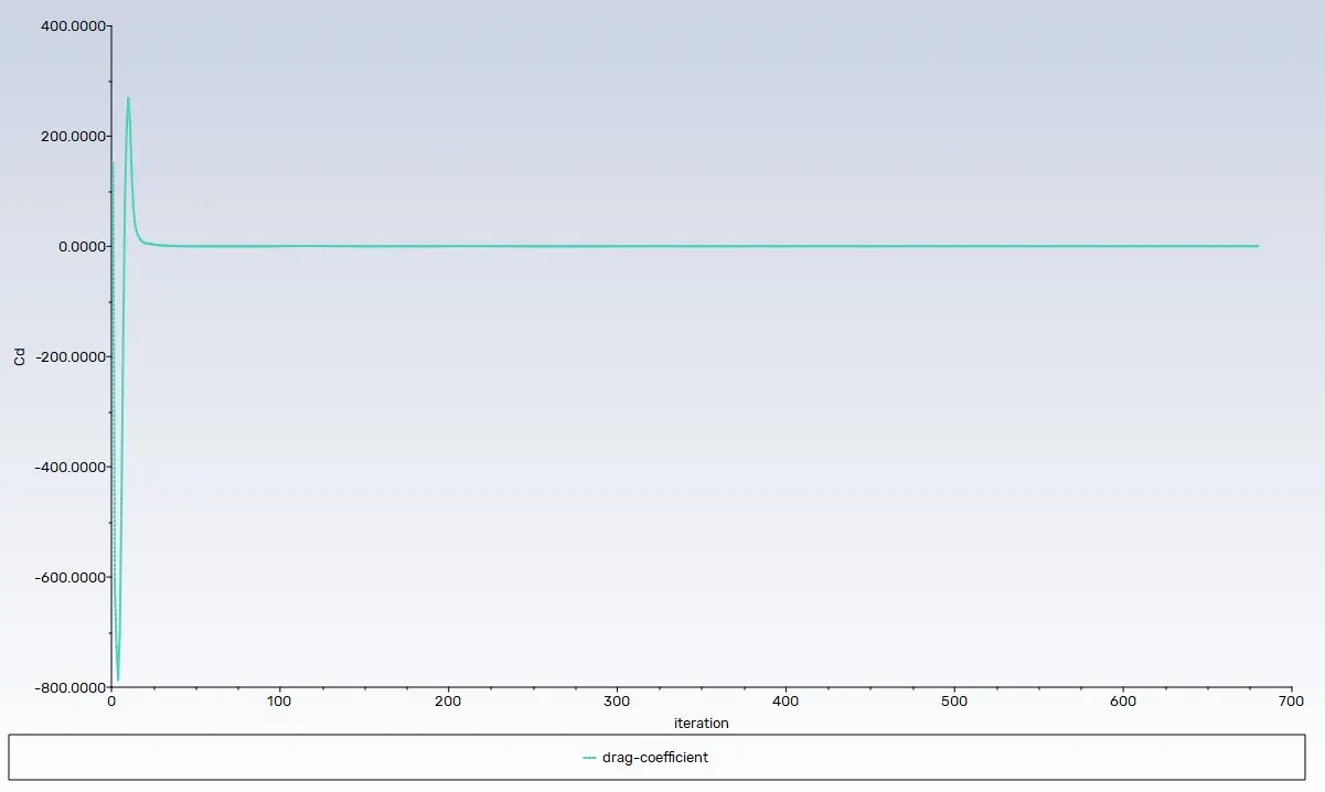
Drag co-efficient plot:
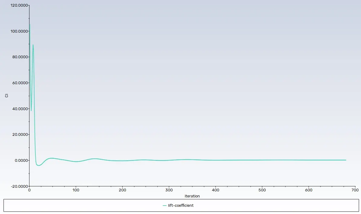
Lift co-efficient plot:
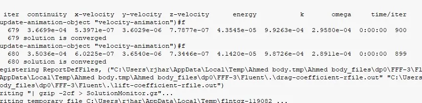
Convergence:
Velocity vector contour:
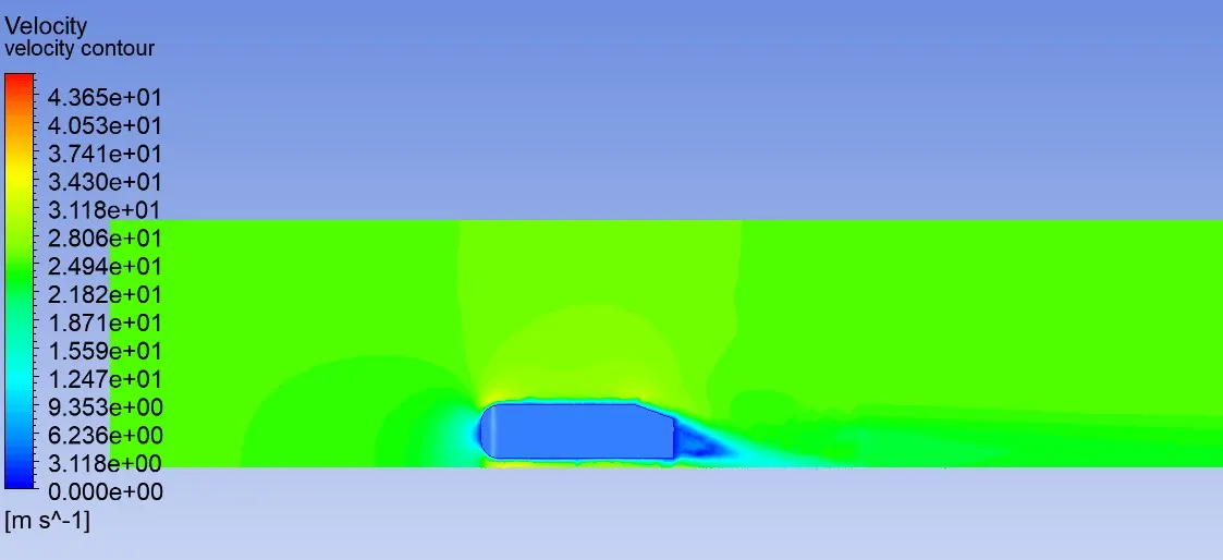
Streamline velocity:
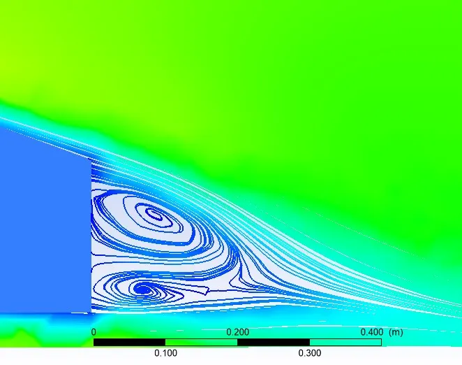
Velocity contour across XY plane (wake region)
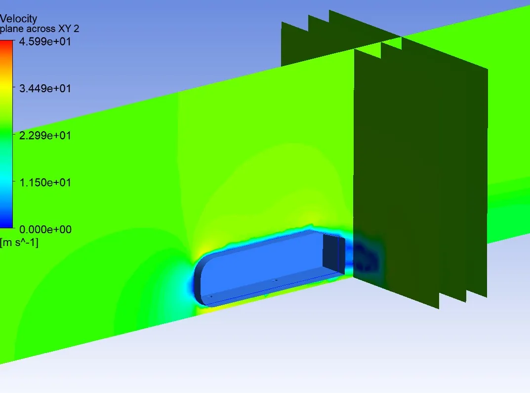
X - 0.106 m from back of the car
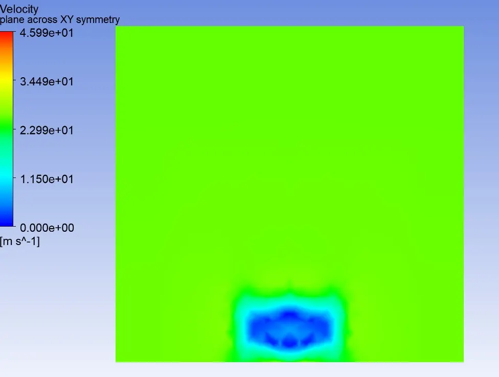
X - 0.300 m from back of the car
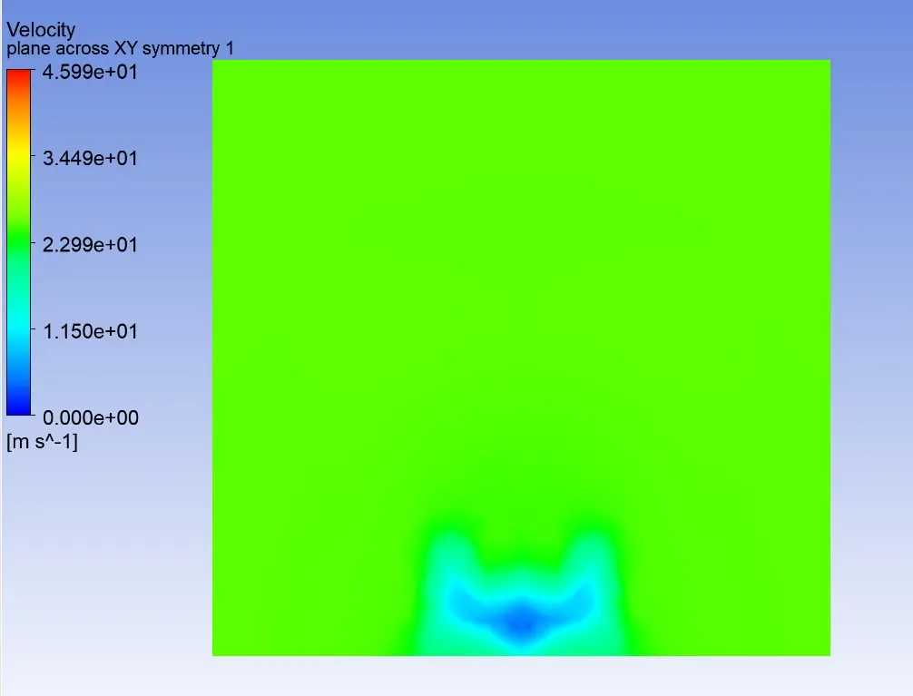
X - 0.450 m from back of the car
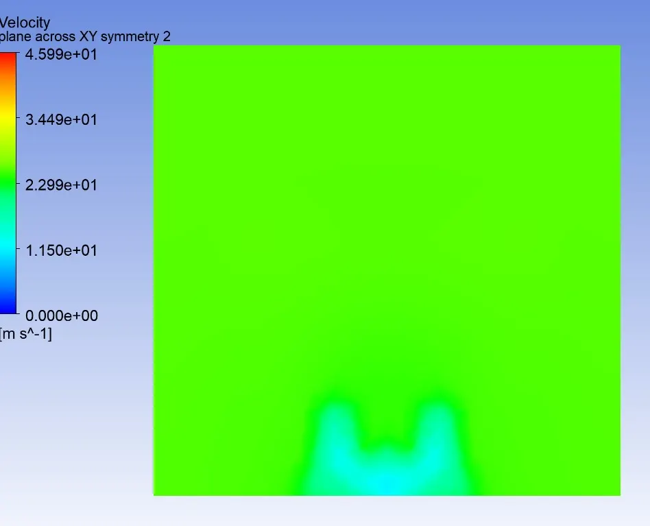
Pressure contour along XY plane:
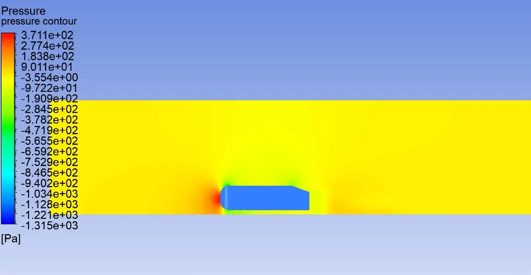
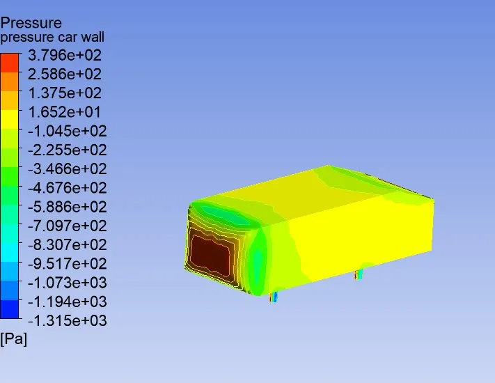
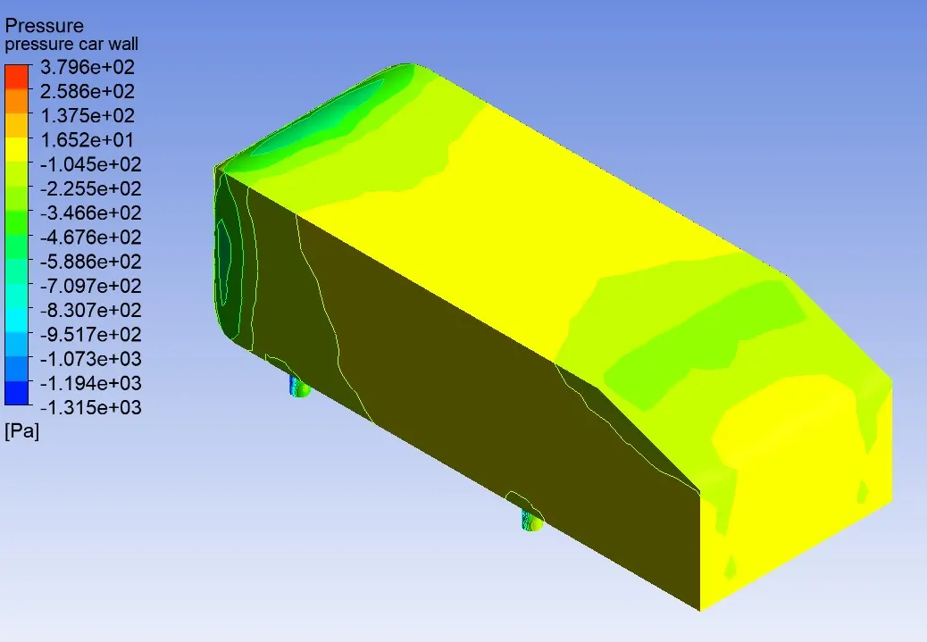
Pressure contour in car wall:
Point of separation in Fluid Flow:
The separation point in boundary layer theory is a critical location where the boundary layer detaches from the surface of a body.
Reynolds number (Re) is the ratio of inertial forces to viscous forces
High Re: Inertia dominates.
Low Re: Viscosity dominates.
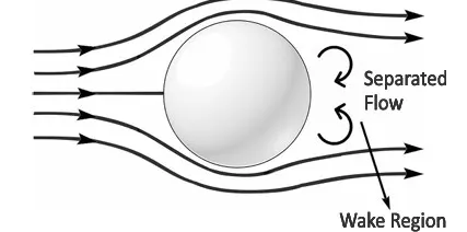
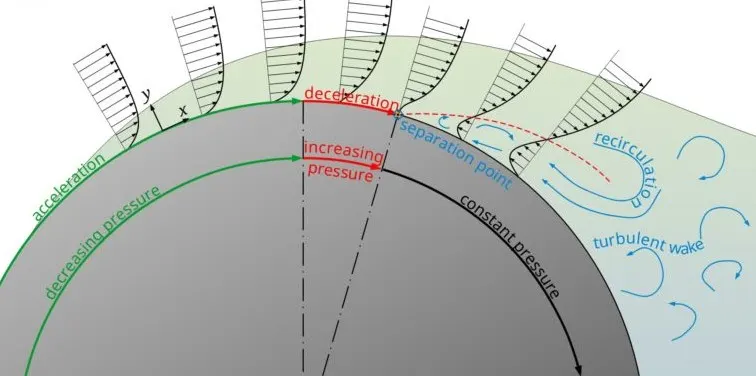
- Near the body surface, the fluid particles slow down due to viscous effects (no-slip condition), forming a velocity gradient — this is the boundary layer.
- The pressure gradient acting against the actual direction of flow is called adverse pressure gradient.
- In regions with an adverse pressure gradient (i.e., pressure increases in the direction of flow), the fluid within the boundary layer loses momentum.
- A point arises where the momentum loss is so severe that the fluid can no longer move forward — the velocity at the wall becomes zero and starts to reverse. This is the separation point.
- Beyond the separation point, flow reverses direction, forming a recirculation zone.
- Negative gauge pressure develops in the wake region due to this reverse flow and low-momentum fluid.
- This region typically has low pressure, contributing significantly to pressure drag.
Effect of flow separation in race cars:

- from the drag equation it can be seen that the drag force is in proportion to the square of the speed.
- This implies that the resistance due to air increases exponentially as the speed of the body increases.
- Flow separation location determines the size of the wake area and amount of aero dynamic drag is determined accordingly.
- When the air moving over the vehicle is separated at the rear end, it leaves a larger low pressure turbulent region behind the vehicle known as wake.
- This wake contributes to the formation of pressure drag.
- To achieve the optimized drag for the vehicle, the research is being carried out on these certain add on aerodynamic devices to reduce the resistance offered by wind and improve the efficiency of the vehicle.
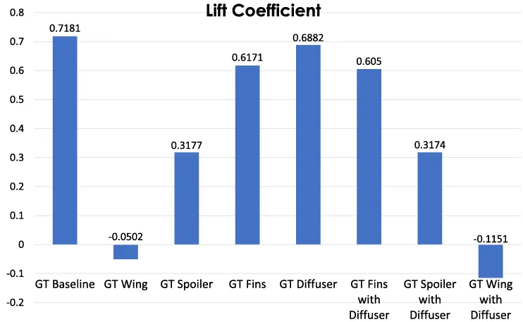
Research paper study: Drag reduction by application of aerodynamic devices in a race car
Types of aerodynamic devices:
- Rear wing
- Spoiler
- diffuser
- fins
Spoiler:
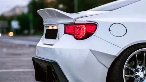
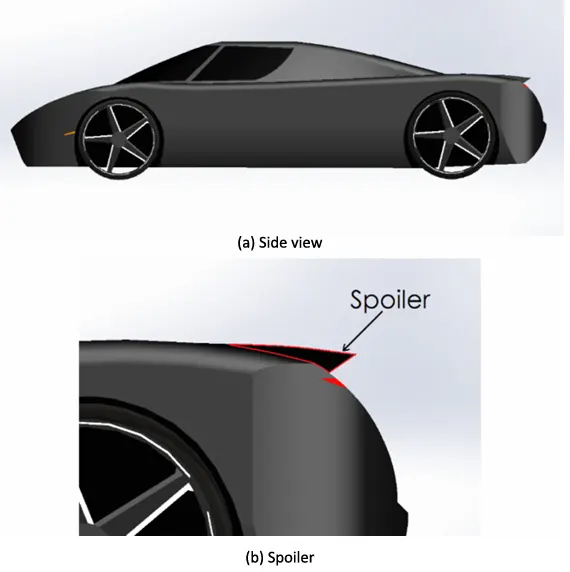
- Spoiler is one of the most widely used and important aerodynamic devices in automotive domain.
- Its main purpose is to "spoil" the unwanted airflow and channel the airflow in order, which helps in reducing the drag.
- However, the actual use of spoiler is noticed at higher speeds approximately above 120 km/hr.
- Commerical vehicles usually adopt it to increase the design appeal of the vehicle, which provides little or no aerodynamics advantages.
- Thus, mostly high-performance vehicle adapts it to achieve higher speed.
- The low-pressure zone behind the vehicle is reduced, thus less turbulence is created which subsequently leads to drag reduction.
Rear wing:
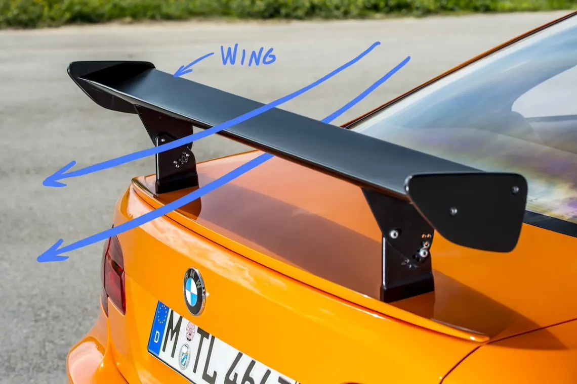
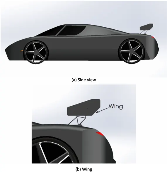
- The wing is another essential aerodynamic device often used by race cars.
- A rear wing may look like spoiler but is different in its functioning.
- It is shaped like a wing of an airplane turned upside down.
- Its main objective is to provide sufficient downforce or negative lift so that the vehicle has increased traction and vehicle doesn't lift off at higher speeds.
- It also allows to corner faster and provides stability at high speeds.
- But using a wing may add up the drag to the vehicle body.
- Thus, for any amount of lift gained, drag also increases.
- It is generally regarded as tradeoff between drag and lift.
Diffuser:
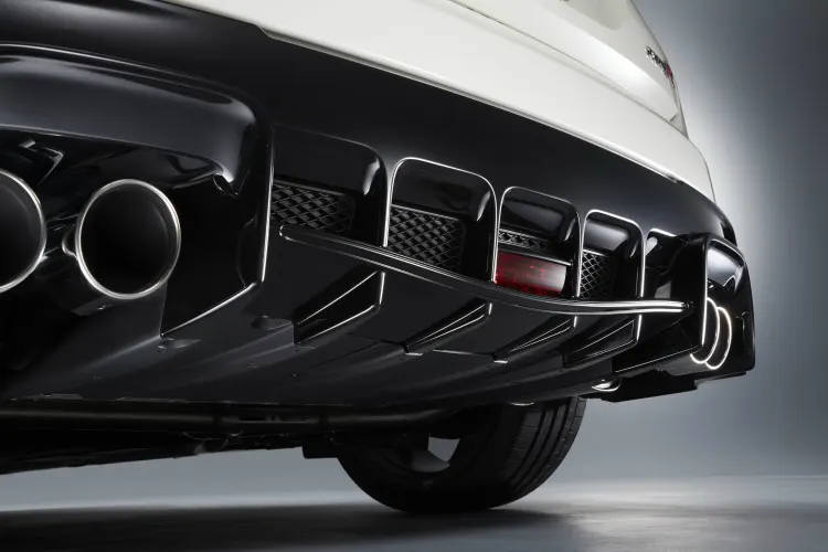
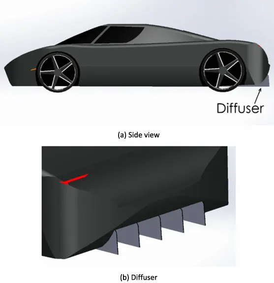
- The diffuser is one of the prominent aerodynamic devices found in formula 1 cars.
- The wide versatility offered by diffusers has found its way down to high-speed production vehicles.
- Diffusers are capable of reducing drag and increasing downforce for driving cars.
- The role of diffusers is to expand the flow from underneath the car to the rear and this in turn produces a pressure potential, which accelerate the flow underneath the car, resulting in reduced pressure.
- The principle behind the working of diffuser is based upon bernoulli's principle which states that " a slow-moving fluid will exert greater pressure than fast moving fluid".
- Thus, the role of diffuser is to accelerate the flow of air beneath the car so that less pressure is exerted in comparison to the outer body flow.
- This serves in ejecting out air from below the car.
- The diffuser then lightens this high-speed air down to normal speed and helps fill the area behind the car, making the entire underbody a more robust downforce and importantly reducing the drag on the vehicle,
Fins:
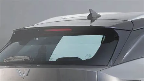
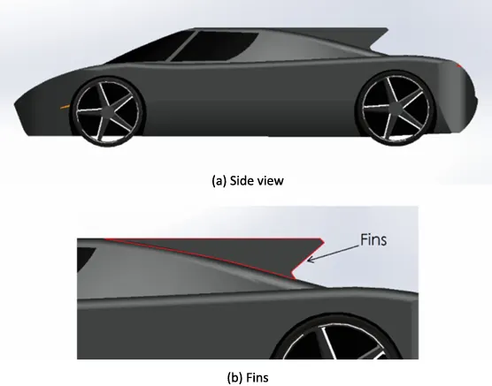
- Small vertical or angled surfaces placed strategically (e.g., sides, roof, near rear window).
- Direct airflow,
- Delay flow separation,
- Sometimes generate vortices to energize the boundary layer.
- Can reduce drag by controlling flow separation.
- May slightly increase drag if not designed properly but are generally beneficial for stability and flow management.
CFD study on above research paper:
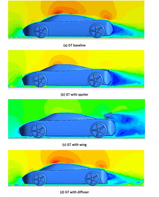
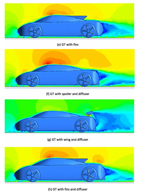
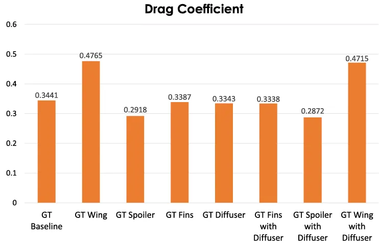
Velocity contour for different cases
Conclusion:
- This study investigated the aerodynamic behaviour of ahmed body using two turbulence models K-epsilon standard and K omega SST, across four cases varying y+ values.
- The k-epsilon standard model was evaluated with wall y+ values of 50, 150, 290.
- while k-omega SST model was tested with a fine near wall resolution (Y+ =1)
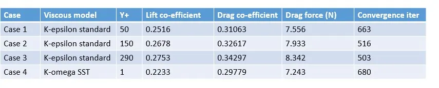
- Result shows that as y+ increased in k-epsilon model, the drag co-efficient and drag force also increased, indicating that coarse mesh (higher Y+) tend to over predict drag due to poor near wall resolution.
- The k-omega SST model with Y+ =1 predicted the lowest drag co-efficient and shows a larger wake region, highlighting its superior capability to resolve near wall and separated flows.
- The SST model also showed better representation of boundary layer behaviour, separation and flow reattachment features critical in bluff body simulation.
- The wake length and pressure drag predicition were significantly affected by turbulence model and wall treatment.
- In conclusion, K-omega SST model with near wall mesh (Y+ =1) is recommended for accurate drag predicition and wake analysis in external aerodynamics simulation like ahmed body.
- However, for cases with limited computational resources, the k-epsilon with wall function (30<Y+<300) can still provide acceptable results though with reduced fidelity in separation and wake region.